Analyze SINR in 6G FR3 Network Using Digital Twin
This example shows how to use digital twin techniques to analyze the signal-to-interference-plus-noise ratio (SINR) performance in a 6G FR3 network. It selects a geographical area of interest served by a base station (gNB) and randomly places user equipment (UE) terminals within this area. The analysis also accounts for interfering base stations. By employing ray tracing techniques, the example calculates the SINR for each UE.
Specify System Parameters
Specify the top-level parameters to use in the simulation. Set the carrier frequency to a value within the FR3 range.
nUEs = 20;              % Number of UEs
fc = 14e9;              % Carrier frequency
PtxdBm = 40;            % gNB transmit power in dBm
PtxInterfdBm = 43;      % Interfering gNB transmit power in dBm
Noc = -145;             % dBm/Hz from 38.101
NRB = 52;               % Number of resource blocks
maxNumReflections = 3;  % Maximum number of ray tracing reflections
maxNumDiffractions = 1; % Maximum number of ray tracing diffractions
txArraySize = [4 4];    % Number of antennas (rows, columns) in transmitter (gNB) rectangular array
rxArraySize = [2 2];    % Number of antennas (rows, columns) in receiver (UE) rectangular array

rng("default");         % Random number generator default settings for result reproducibility
Specify Map Filename
Specify the name of an OpenStreetMap [1] file that contains data for several city blocks in Chicago.
filename = "chicago.osm";Specify Area of Interest
Specify the latitude and longitude corner points of the region of interest.
latROILim = [41.8845 41.8781];
lonROILim = [-87.6354 -87.6279];
Create an instance of the region of interest to manage the map and buildings.
ROI = RegionOfInterest(filename,latROILim,lonROILim);
Generate Random Drops in Region of Interest
Generate random UE drops with a uniform distribution in the region of interest avoiding buildings. The UEs are located on the streets.
ueLocations = ROI.GenerateRandomDrops(nUEs);
Generate a 2-D view showing the random UE locations within the region of interest, including the buildings. Later, the example uses Site Viewer for a 3-D view of the geographic area to perform ray tracing analysis.
% Plot generated UE location points on map
ROI.plotMap(true,ueLocations)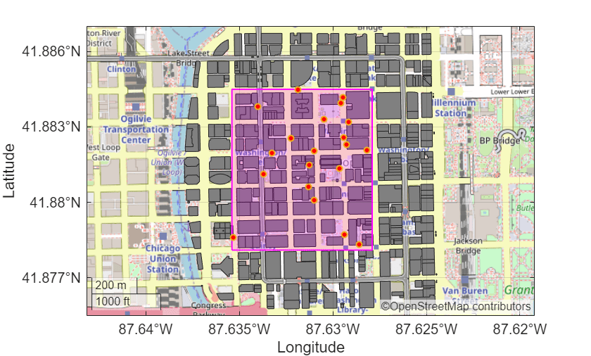
Open Site Viewer
Import the buildings into Site Viewer, a 3-D visualization tool that enables you to locate transmitters and receivers and perform ray tracing analysis.
if exist("viewer","var") && isvalid(viewer) % Viewer handle exists and viewer window is open
    clearMap(viewer);
else
    viewer = siteviewer(Basemap="openstreetmap",Buildings=filename);
end
Create gNB
Model the gNB as a txsite (Antenna Toolbox) object.
gNBLatLon = [41.881696 -87.629566];
lambda = physconst("LightSpeed")/fc;
txArray = phased.URA(Size=txArraySize,ElementSpacing=0.5*lambda);
PtxW = db2pow(PtxdBm-30);
tx = txsite(Latitude=gNBLatLon(1),Longitude=gNBLatLon(2), ...
    TransmitterPower=PtxW, ...
    TransmitterFrequency=fc, ...
    Antenna=txArray, ...
    AntennaAngle=90);

show(tx)
Create UEs in Random Drop Locations
Model the UEs as rxsite (Antenna Toolbox) objects in the locations of the random drops.
% Create all rxsites
rx = rxsite(Latitude=ueLocations(:,1),Longitude=ueLocations(:,2));
% Assign arrays to each rxsite
for n = 1:nUEs
    rx(n).Antenna = phased.URA(Size=rxArraySize,ElementSpacing=0.5*lambda);
end
Perform Ray Tracing Analysis
Create a ray tracing propagation model. Configure the model with the maximum number of reflections and diffractions.
pm = propagationModel("raytracing",MaxNumReflections=maxNumReflections,MaxNumDiffractions=maxNumDiffractions);Perform ray tracing analysis between the gNB and each UE. Calculate the propagation paths and return the result as a cell array of comm.Ray objects.
rays = raytrace(tx,rx,pm);
Calculate Precoding Weights
For the links between the gNB and each UE, calculate the transmitter and receiver precoding (digital beamforming) and combining weights by using singular value decomposition (SVD). Use a comm.RayTracingChannel System object™ to obtain the channel impulse response and the channel matrix.
% Carrier object to obtain sampling rate and OFDM FFT size
carrier = pre6GCarrierConfig(NSizeGrid=NRB);

% Calculate channel matrices using SVD
H = calculateChannelMatrix(carrier,tx,rx,rays);

% Calculate precoding (digital beamforming) and combining weights for all gNB to UE links
[Wrx,S,Wtx] = pagesvd(H);
Calculate UEs Received Signal Power
Calculate the received signal power for all UEs. Account for the precoding and combining gains in the transmitter and receiver arrays.
% UE received signal power (dBm)
ueSignalPowerdBm = calculateSignalPower(tx,rx,rays,Wtx,Wrx);

% UE received signal power (W)
ueSignalPowerW = dBm2W(ueSignalPowerdBm);
Create Interfering gNBs
Specify the locations of the interfering gNBs and set their transmit power. For simplicity, assume the interfering base stations use an isotropic antenna.
interfBS = [41.884085,-87.637310;
            41.885208,-87.625557;
            41.877766,-87.635363;
            41.877684,-87.625858];
txInterf = txsite(Latitude=interfBS(:,1),Longitude=interfBS(:,2), ...
    TransmitterFrequency=fc, ...
    TransmitterPower=dBm2W(PtxInterfdBm));

show(txInterf)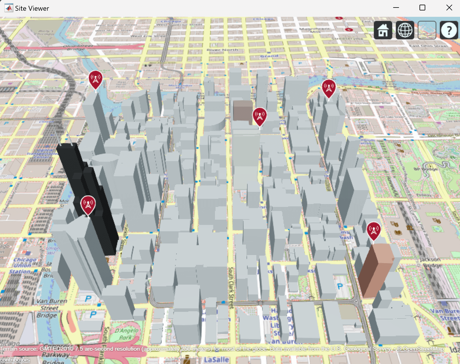
Calculate UEs Interfering Power
For all UEs, calculate the received power from all the interfering base stations. Account for the combining weights that the UEs use to receive the signal of interest.
% Assign MIMO combining weights to each UE before calculating the received
% interfering power
isLoS = zeros(nUEs,1);
for ueIdx=1:nUEs
    wrx = Wrx(:,1,ueIdx).'; % Weights from strongest singular value
    rx(ueIdx).Antenna.Taper = conj(wrx);
    isLoS(ueIdx) = any([rays{ueIdx}.LineOfSight]);
end

% Calculate interfering power for all UEs from each interfering gNB
numInterf = length(txInterf);
interfPowerdBm = zeros(nUEs,numInterf);
for n=1:numInterf
    interfPowerdBm(:,n) = sigstrength(rx,txInterf(n),pm);
end

% Interference power per UE per interfering base station
interfPowerW = dBm2W(interfPowerdBm);

% Combine the interference power for all interfering base stations per UE
% (in W)
ueInterfPowerW = sum(interfPowerW,2);
Calculate SINR
For each UE, calculate the SINR and display the results on the map. In this example, the definition of SINR is the ratio between the signal power and the interference and noise power in the time domain, at the input of the receiver. It includes the effect of precoding and combining at both the gNB and UE.
% Noise power
noisePowerdBm = Noc+10*log10(carrier.NSizeGrid*12*carrier.SubcarrierSpacing*1e3);
noisePowerW = dBm2W(noisePowerdBm);

% Calculate SINR
SINR = 10*log10(ueSignalPowerW./(ueInterfPowerW+noisePowerW));

% Result table
varNames = ["UE" "UE signal power (dBm)" "LOS" "Interf power (dBm)" "Noise+Interf (dBm)" "SINR"];
SINRTable = table((1:nUEs).',ueSignalPowerdBm,isLoS,W2dBm(ueInterfPowerW),W2dBm(ueInterfPowerW+noisePowerW),SINR,VariableNames=varNames);
disp(SINRTable);
    UE    UE signal power (dBm)    LOS    Interf power (dBm)    Noise+Interf (dBm)     SINR
    __    _____________________    ___    __________________    __________________    _______

     1           -42.686            1          -102.73               -75.279           32.594
     2           -64.508            0          -63.488                -63.21          -1.2982
     3           -101.77            0          -105.78               -75.283          -26.484
     4           -48.153            0          -73.862               -71.506           23.353
     5           -91.348            0          -86.367               -74.961          -16.387
     6           -49.324            1           -78.02               -73.432           24.108
     7           -52.862            0          -91.649               -75.188           22.326
     8           -52.698            1          -95.988                -75.25           22.553
     9           -98.509            0          -79.936               -74.007          -24.502
    10           -94.463            0          -74.285               -71.747          -22.716
    11           -70.936            0          -110.59               -75.286           4.3495
    12           -84.024            0           -65.41               -64.985          -19.039
    13           -79.678            0          -73.724               -71.426          -8.2529
    14           -97.142            0          -104.42               -75.282          -21.861
    15            -56.74            0          -113.69               -75.287           18.546
    16            -85.54            0          -107.37               -75.285          -10.255
    17           -67.191            1           -69.78               -68.704           1.5122
    18            -96.44            0          -67.574               -66.895          -29.545
    19           -99.777            0          -73.578               -71.339          -28.438
    20           -50.597            1          -95.428               -75.245           24.649
Display the SINR on the map.
ROI.plotMap(true,ueLocations,SINR,[tx.Latitude tx.Longitude],interfBS)

Explore Further
You can investigate the SINR over the whole area of interest by increasing the number of UEs to consider. This figure shows the SINR with 2000 UEs randomly distributed in the area of interest.

References
[1] The osm file is downloaded from https://www.openstreetmap.org, which provides access to crowdsourced map data all over the world. The data is licensed under the Open Data Commons Open Database License (ODbL), https://opendatacommons.org/licenses/odbl/.
Local Functions
function yW = dBm2W(ydBm)
% dBm to W conversion
    yW = 10.^((ydBm-30)/10);
end

function ydBm = W2dBm(yW)
% W to dBm conversion
    ydBm = pow2db(yW)+30;
end

function H = calculateChannelMatrix(carrier,tx,rx,rays)
% Calculate the channel matrices for all links between the gNB and all
% receivers using the result of the ray tracing analysis. The resulting
% channel matrix H is of size nRx-by-nTx-by-nUEs, where nRx and nTx are the
% number of transmit and receive antennas respectively, and nUEs is the
% number of UEs. The channel matrix is obtained using an average in time
% and frequency over a slot.

    % Obtain sampling rate and OFDM FFT size
    ofdmInfo = nrOFDMInfo(carrier);
    fs = ofdmInfo.SampleRate;

    % Number of transmit and receive antennas
    nTx = prod(tx.Antenna.Size);
    nRx = prod(rx(1).Antenna.Size); % Assume all receivers have the same number of antennas

    % Tx power per antenna
    PtxPerAnt = tx.TransmitterPower/nTx;

    % Calculate channel matrix
    nUEs = length(rx);
    H = zeros(nRx,nTx,nUEs);
    for ueIdx=1:nUEs
        if ~isempty(rays{ueIdx})
            % Create channel object
            ch = comm.RayTracingChannel(rays{ueIdx},tx,rx(ueIdx));
            ch.SampleRate = fs;
            ch.NormalizeImpulseResponses = false; % maintain path loss information
            ch.NormalizeChannelOutputs = false;
            ch.ChannelFiltering = false;
            ch.NumSamples = sum(ofdmInfo.SymbolLengths(1:14)); % one slot
            cir = ch(); % channel impulse response
            chInfo = ch.info();

            % OFDM channel response
            pathFilters = chInfo.ChannelFilterCoefficients;
            K = ofdmInfo.Nfft.^2/(carrier.NSizeGrid*12);
            hest = sqrt(nTx)*sqrt(PtxPerAnt)*sqrt(K)*nrPerfectChannelEstimate(carrier,cir,pathFilters.');

            % Average channel response over time and freq
            H(:,:,ueIdx) = squeeze(mean(hest(:,:,:,:),[1 2]));
        end
    end
end

function ueSignalPowerdBm = calculateSignalPower(tx,rx,rays,Wtx,Wrx)
% Calculate the received signal power given a txsite, nUEs rxsites
% (rx), using the rays between the transmitter and receivers. Wtx and Wrx
% are the precoding and combining matrices to consider for the power
% calculation.

    nUEs = length(rx);
    fc = tx.TransmitterFrequency;
    PtxdBm = W2dBm(tx.TransmitterPower);
    ueSignalPowerdBm = zeros(nUEs,1);
    for ueIdx=1:nUEs
        if ~isempty(rays{ueIdx})
            % Precoding and combining weights corresponding to this gNB to
            % UE link
            wtx = Wtx(:,1,ueIdx).'; % Weights from strongest singular value
            wrx = Wrx(:,1,ueIdx).'; % Weights from strongest singular value

            % AoD and AoA angles
            AoD = [rays{ueIdx}.AngleOfDeparture];
            AoD(1,:) = AoD(1,:) - tx.AntennaAngle;
            AoA = [rays{ueIdx}.AngleOfArrival];
            AoA(1,:) = AoA(1,:) - rx(ueIdx).AntennaAngle;

            % Make sure rx array has no taper, as weights are specified as
            % an argument when calling the directivity() function, and not
            % as part of the array taper property.
            rx(ueIdx).Antenna.Taper = 1;

            % Calculate the received signal power per UE
            txDirectivity = directivity(tx.Antenna, fc, wrapTo180(AoD),"Weights",wtx.');
            rxDirectivity = directivity(rx(ueIdx).Antenna, fc, wrapTo180(AoA),"Weights",wrx.');
            rxPowerdBW = PtxdBm - 30 + txDirectivity' + rxDirectivity' - [rays{ueIdx}.PathLoss]; % in dBW
            rxSignalLevel = exp(1i*[rays{ueIdx}.PhaseShift]) .* 10.^(rxPowerdBW/20); % in V
            ueSignalPowerdBm(ueIdx) = W2dBm(abs(sum(rxSignalLevel)).^2); % dBm
        else
            ueSignalPowerdBm(ueIdx) = -Inf;
        end
    end
end
See Also
comm.RayTracingChannel | txsite (Antenna Toolbox) | rxsite (Antenna Toolbox)