Troubleshooting 5G Network Performance with Digital Twin
R2026bUse a 5G network digital twin to investigate and resolve poor throughput in a multi-cell deployment. This example applies ray tracing in a 3-D urban environment to model realistic propagation and inter-cell interference.
Introduction
This example models two gNBs operating in downtown Chicago. Each gNB serves one UE in a synchronized TDD configuration. Both UEs suffer inter-cell interference. The gNBs select MCS based on reference signal measurements (SRS for uplink, CSI-RS for downlink). However, these measurements do not fully represent the inter-cell interference that UEs experience during data transmission. The reference signals experience a higher SINR than the PUSCH/PDSCH, causing the gNBs to select too high an MCS for the channel conditions, resulting in a high BLER.
This example uses a digital twin to diagnose this mismatch and validate a fix: enabling outer-loop link adaptation (OLLA), which adjusts the MCS based on HARQ ACK/NACK feedback until BLER converges to a target.
Specify System Parameters
simulationTime = 0.2;                % Simulation time in seconds
fc = 4.2e9;                          % Carrier frequency (Hz)
PtxgNBdBm = 33;                      % gNB transmit power in dBm
PtxUEdBm = 23;                       % UE transmit power in dBm
NRB = 51;                            % Number of resource blocks
SCS = 30;                            % Subcarrier spacing (kHz)
duplexingMode = "TDD";               % Duplexing mode
maxNumReflections = 2;               % Maximum number of ray tracing reflections
maxNumDiffractions = 1;              % Maximum number of ray tracing diffractions
gNBArrayRectangularDim = [1 2];      % gNB antenna array [rows, columns], each location in the array has two cross-polarized antennas
ueArrayRectangularDim = [1 1];       % UE antenna array [rows, columns], each location in the array has two cross-polarized antennas

% TDD configuration, shared by both cells.
tddConfig = struct('DLULPeriodicity', 2.5, ...
    'NumDLSlots', 2, 'NumDLSymbols', 10, 'NumULSymbols', 0, 'NumULSlots', 2);

% Parameter validation
validategNBArraySize(gNBArrayRectangularDim);
BW = validateNumerology(SCS,NRB);
Calculate and display the simulation length.
wInfo = nrOFDMInfo(NRB,SCS);
slotDuration = 1e-3 / wInfo.SlotsPerSubframe;
nSlots = floor(simulationTime / slotDuration);
disp("Simulation: " +nSlots/wInfo.SlotsPerFrame+" frames = "+ nSlots + " slots (" + simulationTime*1e3 + " ms)")
Simulation: 20 frames = 400 slots (200 ms)
Specify Network Scenario
Specify the name of an OpenStreetMap file [1] with 3-D buildings information. Specify the geographic coordinates (latitude and longitude) of the gNBs and UEs.
fileName = "chicago.osm";

% gNB locations (rooftop deployments)
gNBLocations = [41.876853, -87.626942;   % gNB1
                41.877706, -87.630108];  % gNB2
% gNB array broadside azimuth (0 deg is East) and elevation angles (deg)
gNBArrayAngles = [180, -6;    % (az, el) gNB1
                 -90, -6];   % (az, el) gNB2
gNBArrayHeight = [15 15];              % Antenna height above mounting surface (m)
numgNBs = size(gNBLocations,1);
gNBLabels = "gNB"+string(1:numgNBs);

% UE locations
ueLocations = [41.877474, -87.627943;  % UE1 (served by gNB1)
              41.876909, -87.630235];  % UE2 (served by gNB2)
ueArrayAngles = [0, 0;   % (az, el) UE1
                 100, 0]; % (az, el) UE2
ueArrayHeight = 1.5; % m
numUEs = size(ueLocations,1);
ueLabels = "UE"+string(1:numUEs);

rng("default");
plotNodeLocations("gNB and UE Locations", ...
    gNBLocations,ueLocations,gNBLabels,ueLabels);
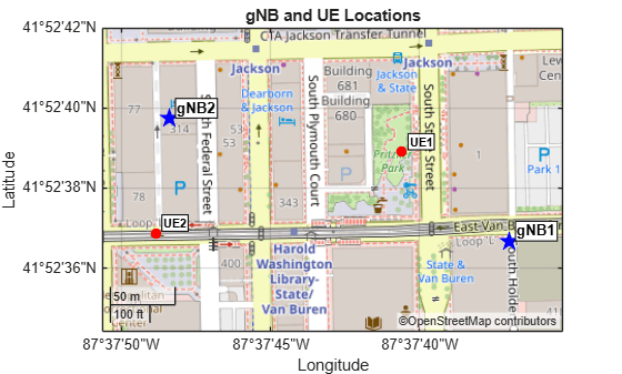
Perform Ray Tracing Analysis
Perform ray tracing analysis, resulting in a set of rays the example uses for channel modeling during network simulation.
Create gNB Sites
Create the gNB sites for ray tracing analysis.
Precalculate the gNB transmit power in watts, the wavelength, and the uplink and downlink carrier frequencies.
% gNB transmit power in watts
PtxW = db2pow(PtxgNBdBm-30);

% Wavelength for array dimensioning
lambda = freq2wavelen(fc);

% Calculate uplink and downlink carrier frequencies
[dlFc,ulFc] = fddCarrierFreq(duplexingMode,fc,BW);
Create the gNB site objects for ray tracing analysis. Each gNB has its own array with the broadside pointing in the direction you specify in gNBArrayAngles.
% Create gNB sites for ray tracing
gnbSites = txsite.empty();
gnbArrays = cell(1,numgNBs);
for n = 1:numgNBs
    gnbArrays{n} = phased.NRRectangularPanelArray(Size=[gNBArrayRectangularDim 1 1], ...
        Spacing=[0.5*lambda*[1 1] 1 1], ...
        ElementSet={phased.NRAntennaElement(PolarizationAngle=45), ...
                    phased.NRAntennaElement(PolarizationAngle=-45)});
    gnbSites(n) = txsite(Name=gNBLabels(n), ...
        Latitude=gNBLocations(n,1), Longitude=gNBLocations(n,2), ...
        TransmitterPower=PtxW, TransmitterFrequency=dlFc, ...
        Antenna=gnbArrays{n}, AntennaHeight=gNBArrayHeight(n), ...
        AntennaAngle=gNBArrayAngles(n,:)');
end
Create UE Sites
Create the UE site objects for ray tracing analysis.
% Create UE dipole antenna elements
ueAnt1PolAngle = 0;                                           % First polarization angle in degrees
ueAnt2PolAngle = 90;                                          % Second polarization angle in degrees
% Polarization direction vectors: 0 deg vertical, 90 deg horizontal
polVector1 = [0; sind(ueAnt1PolAngle); cosd(ueAnt1PolAngle)];
polVector2 = [0; sind(ueAnt2PolAngle); cosd(ueAnt2PolAngle)];
% Create short dipole antenna elements
pol1AntElement = phased.ShortDipoleAntennaElement(AxisDirection='Custom',CustomAxisDirection=polVector1);
pol2AntElement = phased.ShortDipoleAntennaElement(AxisDirection='Custom',CustomAxisDirection=polVector2);

% Create UE sites for ray tracing
ueSites = rxsite.empty();
ueArrays = cell(1,numUEs);
for n = 1:numUEs
    ueArrays{n} = phased.NRRectangularPanelArray(Size=[ueArrayRectangularDim 1 1], ...
        Spacing=[0.5*lambda*[1 1] 1 1], ...
        ElementSet={pol1AntElement,pol2AntElement});
    ueSites(n) = rxsite(Name=ueLabels(n), ...
        Latitude=ueLocations(n,1), Longitude=ueLocations(n,2), ...
        Antenna=ueArrays{n}, AntennaHeight=ueArrayHeight, ...
        AntennaAngle=ueArrayAngles(n,:)');
end
Open Site Viewer to view the map and buildings, and display the gNB and UE locations.
% Site Viewer
if exist('viewer','var') && isvalid(viewer) % viewer handle exists and viewer window is open
    clearMap(viewer);
else
    viewer = siteviewer(Basemap="openstreetmap",Buildings=fileName);
end
show(ueSites)
show(gnbSites)
Perform Ray Tracing Analysis
Perform ray tracing analysis between each gNB and all UEs. Create a ray tracing propagation model with the specified maximum number of reflections and diffractions. You can specify other parameters associated with ray tracing in this propagation model object.
% Ray tracing (use the OSM file for 3-D building geometry)
pm = propagationModel("raytracing", ...
    MaxNumReflections=maxNumReflections, ...
    MaxNumDiffractions=maxNumDiffractions, MaxRelativePathLoss=Inf);
The gnbSites and ueSites are arrays of txsite and rxsite objects respectively. You can use them to perform the downlink ray tracing analysis. To perform the uplink ray tracing analysis, create txsite and rxsite objects for UEs and gNBs respectively. You can also use these objects to create the uplink ray tracing channel models.
[txueUL,rxgNBUL] = createULSites(gnbSites,ueSites,db2pow(PtxUEdBm-30),ulFc);
Perform the ray tracing analysis between each gNB and each UE. For TDD, the example assumes channel reciprocity, where the DL and UL channels are the same. Therefore, the example skips the UL ray tracing calculation. Instead, it uses the information in the DL rays to calculate the UL rays.
raysDL = cell(1,numgNBs);
raysUL = cell(1,numgNBs);
for n = 1:numgNBs
    raysDL{n} = raytrace(gnbSites(n),ueSites,pm);
    raysUL{n} = dl2ulRays(raysDL{n});
end

% Cartesian coordinates
gNBxyz = zeros(numgNBs,3);
for n = 1:numgNBs
    gNBxyz(n,:) = latLonToCartesianFlatEarth(gNBLocations(n,:), ...
        gnbSites(n).elevation+gnbSites(n).AntennaHeight, gNBLocations(1,:));
end
uesxyz = zeros(numUEs,3);
for n = 1:numUEs
    uesxyz(n,:) = latLonToCartesianFlatEarth(ueLocations(n,:), ...
        ueSites(n).elevation+ueSites(n).AntennaHeight, gNBLocations(1,:));
end
Simulate Network
Set up and perform the network simulation using the results of the ray tracing analysis.
Initialize network simulator.
networkSimulator = wirelessNetworkSimulator.init;
Create gNBs.
% Convert the gNB and UE array angles to node array orientations
gNBOrientations = arrayAnglesToOrientation(gNBArrayAngles);
ueOrientations = arrayAnglesToOrientation(ueArrayAngles);

gnbs = nrGNB.empty(); % Empty nrGNB array, clear nodes from any previous run
for n = 1:numgNBs
    gnbs(n) = nrGNB(Position=gNBxyz(n,:), ...
        TransmitAntennaArray=gnbArrays{n}, ReceiveAntennaArray=gnbArrays{n}, ...
        TransmitArrayOrientation=gNBOrientations(:,n), ReceiveArrayOrientation=gNBOrientations(:,n), ...
        CarrierFrequency=fc, ChannelBandwidth=BW, NumResourceBlocks=NRB, ...
        SubcarrierSpacing=SCS, DuplexMode=duplexingMode, ...
        DLULConfigTDD=tddConfig, ...
        TransmitPower=PtxgNBdBm, NoiseFigure=6, ReceiveGain=6, ...
        SRSPeriodicityUE=10, ...
        PHYModel="abstract-phy", Name=gNBLabels(n));
end
Create UEs.
ues = nrUE.empty(); % Empty nrUE array, clear nodes from any previous run
for n = 1:numUEs
    ues(n) = nrUE(Position=uesxyz(n,:), ...
        TransmitAntennaArray=ueArrays{n}, ReceiveAntennaArray=ueArrays{n}, ...
        TransmitArrayOrientation=ueOrientations(:,n), ReceiveArrayOrientation=ueOrientations(:,n), ...
        TransmitPower=PtxUEdBm, NoiseFigure=6, ReceiveGain=6, Name=ueLabels(n));
end
Create channel registry.
rtChanReg = createChannelRegistry(NRB,SCS,gnbs,ues, ...
    raysDL,raysUL,gnbSites,ueSites,txueUL,rxgNBUL);
Disable link adaptation for this first run. This makes the gNB select the MCS and number of layers based on reference signal measurements: SRS for uplink, CSI-RS for downlink. These measurements reflect channel conditions during the reference signal symbols.
linkAdaptation = false;
Run network simulation.
[logTables,ueInfo,kpiManager] = runNetworkSimulation(networkSimulator, simulationTime, ...
    gnbs, ues, rtChanReg, distance(gnbSites,ueSites), linkAdaptation);
gNB1: serves UE1 gNB2: serves UE2
Calculate and display the throughput and BLER for the whole simulation.
windowSize = nSlots; % slots

kpis1 = getBLERandThroughput(kpiManager,simulationTime,slotDuration,windowSize,gnbs(1),ues(1));
kpis2 = getBLERandThroughput(kpiManager,simulationTime,slotDuration,windowSize,gnbs(2),ues(2));

kpisTable = table([ues.Name]',[kpis1.dlThput; kpis2.dlThput],[kpis1.dlBLER; kpis2.dlBLER],[kpis1.ulThput; kpis2.ulThput],[kpis1.ulBLER; kpis2.ulBLER], ...
    VariableNames=["UE","DL Thput (Mbps)","DL BLER (%)","UL Thput (Mbps)","UL BLER (%)"]);
disp(kpisTable)
     UE      DL Thput (Mbps)    DL BLER (%)    UL Thput (Mbps)    UL BLER (%)
    _____    _______________    ___________    _______________    ___________

    "UE1"        108.73                0           38.737           50.633
    "UE2"        44.431           16.102           71.214                0
The system is designed to achieve a BLER of around 10%. In this case, the uplink BLER for UE1 and the downlink BLER for UE2 are above the target. For a more detailed view of the BLER and throughput over time, you can use the kpiManager object.
Calculate how the throughput and BLER evolve throughout the simulation using an averaging window of 20 slots.
windowSize = 20; % slots
kpis1vsTime = getBLERandThroughput(kpiManager,simulationTime,slotDuration,windowSize,gnbs(1),ues(1));
kpis2vsTime = getBLERandThroughput(kpiManager,simulationTime,slotDuration,windowSize,gnbs(2),ues(2));

tl = plotKPIs(kpis1vsTime.kpiSlotRange,[kpis1vsTime.dlBLER; kpis2vsTime.dlBLER],[kpis1vsTime.dlThput; kpis2vsTime.dlThput],...
                                       [kpis1vsTime.ulBLER; kpis2vsTime.ulBLER],[kpis1vsTime.ulThput; kpis2vsTime.ulThput],{"UE1", "UE2"});
title(tl,"BLER and Throughput (window="+windowSize+" slots). No link adaptation");
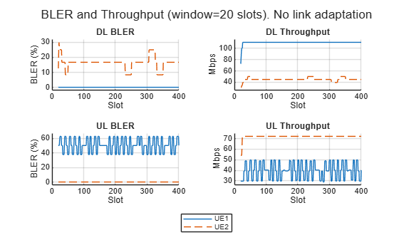
The UL BLER for UE1 is ~50%. Investigate the SINR, MCS and number of layers for UE1.
plotSINRandMCS(logTables,ueInfo(ueInfo.Label=="UE1",:),wInfo);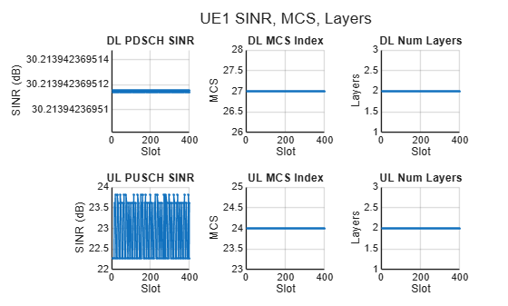
The UL SINR and MCS for UE1 are high for a BLER of 50%. This indicates that the gNB overestimates the quality of the channel. The gNB uses the reference signals to estimate the SINR, then uses this value to calculate the MCS and number of layers required to achieve a BLER of around 10%. However, the SINR experienced by the data channel can be different from the SINR experienced by the reference signals. You can verify this by extracting and plotting both SINR measurements from the log tables.
plotRefVsDataSINR(logTables,ueInfo,wInfo);
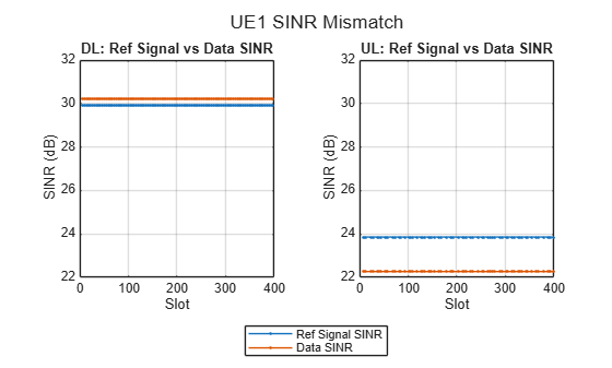
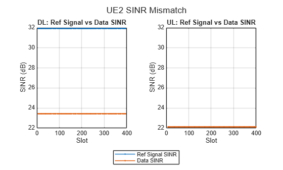
For the UE1 uplink and UE2 downlink cases there is a mismatch between the SINR obtained using reference signals and the SINR experienced by the data channel. These are the links with a BLER above the 10% target.
Both gNBs use identical reference signal configurations, therefore they overlap in time and frequency and interfere with each other. However, the interference power differs between reference signals and data due to precoding: CSI-RS is transmitted without beamforming, so inter-cell CSI-RS interference is weak. PDSCH, on the other hand, is beamformed toward the intended UE, concentrating energy in a direction that can cause interference to other UEs. The scheduler uses the CSI-RS-based SINR (which underestimates interference) to select MCS, resulting in a value too high for the channel conditions.
You can observe the following from the SINR plots:
UE1 DL: High SINR and small mismatch between the SINR from reference signals and data, resulting in 0 BLER
UE1 UL: The SRS-based SINR overestimates the PUSCH SINR. This causes an overly aggressive MCS selection, resulting in a 50% BLER.
UE2 DL: The CSI-RS SINR is higher than the PDSCH SINR. This is caused by the neighboring gNB's beamformed PDSCH, which creates interference, and results in a BLER above the 10% target.
UE2 UL: The SINR is high and the SRS and PUSCH experience similar interference levels.
Simulate Network with Link Adaptation
You can enable OLLA to adjust the MCS based on block decoding failures (HARQ NACK). After each HARQ NACK, OLLA increases a SINR back-off by a step up value (StepUp); after each ACK, it decreases by a step down amount (StepDown). This drives the MCS down until BLER converges to the target: StepDown/(StepUp+StepDown) = 10%.
Initialize network simulator.
networkSimulator = wirelessNetworkSimulator.init;
Create gNBs.
for n = numgNBs:-1:1
    gnbs(n) = nrGNB(Position=gNBxyz(n,:), ...
        TransmitAntennaArray=gnbArrays{n}, ReceiveAntennaArray=gnbArrays{n}, ...
        TransmitArrayOrientation=gNBOrientations(:,n), ReceiveArrayOrientation=gNBOrientations(:,n), ...
        CarrierFrequency=fc, ChannelBandwidth=BW, NumResourceBlocks=NRB, ...
        SubcarrierSpacing=SCS, DuplexMode=duplexingMode, ...
        DLULConfigTDD=tddConfig, ...
        TransmitPower=PtxgNBdBm, NoiseFigure=6, ReceiveGain=6, ...
        SRSPeriodicityUE=10, ...
        PHYModel="abstract-phy", Name=gNBLabels(n));
end
Create UEs.
for n = numUEs:-1:1
    ues(n) = nrUE(Position=uesxyz(n,:), ...
        TransmitAntennaArray=ueArrays{n}, ReceiveAntennaArray=ueArrays{n}, ...
        TransmitArrayOrientation=ueOrientations(:,n), ReceiveArrayOrientation=ueOrientations(:,n), ...
        TransmitPower=PtxUEdBm, NoiseFigure=6, ReceiveGain=6, Name=ueLabels(n));
end
Create channel registry.
rtChanReg = createChannelRegistry(NRB, SCS, gnbs, ues, ...
    raysDL, raysUL, gnbSites, ueSites, txueUL, rxgNBUL);
Enable link adaptation.
linkAdaptation = true;
Run network simulation.
[logTablesLA,~,kpiManagerLA] = runNetworkSimulation(networkSimulator, simulationTime, ...
    gnbs, ues, rtChanReg, distance(gnbSites,ueSites), linkAdaptation);
gNB1: serves UE1 gNB2: serves UE2
Calculate and display the throughput and BLER.
windowSize = nSlots; % slots
kpis1LA = getBLERandThroughput(kpiManagerLA,simulationTime,slotDuration,windowSize,gnbs(1),ues(1));
kpis2LA = getBLERandThroughput(kpiManagerLA,simulationTime,slotDuration,windowSize,gnbs(2),ues(2));

kpisTableLA = table([ues.Name]',[kpis1LA.dlThput; kpis2LA.dlThput],[kpis1LA.dlBLER; kpis2LA.dlBLER],[kpis1LA.ulThput; kpis2LA.ulThput],[kpis1LA.ulBLER; kpis2LA.ulBLER], ...
    VariableNames=["UE","DL Thput (Mbps)","DL BLER (%)","UL Thput (Mbps)","UL BLER (%)"]);
disp(kpisTableLA)
     UE      DL Thput (Mbps)    DL BLER (%)    UL Thput (Mbps)    UL BLER (%)
    _____    _______________    ___________    _______________    ___________

    "UE1"        108.73                0            60.87           11.392
    "UE2"        47.672           10.169           62.847           10.127
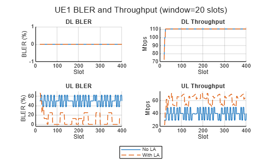
With OLLA enabled, the BLER values are closer to the 10% target for the links that were previously suffering high BLER.
Check the network performance with and without OLLA for UE1.
windowSize = 20; % slots
kpis1vsTimeLA = getBLERandThroughput(kpiManagerLA,simulationTime,slotDuration,windowSize,gnbs(1),ues(1));

tl = plotKPIs(kpis1vsTime.kpiSlotRange,[kpis1vsTime.dlBLER; kpis1vsTimeLA.dlBLER],[kpis1vsTime.dlThput; kpis1vsTimeLA.dlThput],...
                                       [kpis1vsTime.ulBLER; kpis1vsTimeLA.ulBLER],[kpis1vsTime.ulThput; kpis1vsTimeLA.ulThput],{"No LA", "With LA"});
title(tl,"UE1 BLER and Throughput (window="+windowSize+" slots)");
Explore the SINR, MCS and number of layers for UE1 with and without the use of OLLA.
plotSINRandMCS({logTables,logTablesLA},ueInfo(ueInfo.Label=="UE1",:),wInfo,["No LA","With LA"]);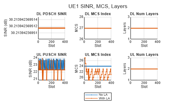
The comparison plots show the effect of OLLA on downlink and uplink for UE1:
UE1 DL: This link had a high SINR and was already at MCS 27 (the maximum). OLLA has no effect here since it cannot select a higher MCS. The BLER is unchanged.
UE1 UL: OLLA responds to the stream of NACKs by stepping down the MCS. After a convergence period of a few slots, the MCS stabilizes and the BLER drops to ~10%. The throughput improves accordingly as most transport blocks are decoded successfully.
Check the network performance with and without OLLA for UE2.
kpis2vsTimeLA = getBLERandThroughput(kpiManagerLA,simulationTime,slotDuration,windowSize,gnbs(2),ues(2));

tl = plotKPIs(kpis2vsTime.kpiSlotRange,[kpis2vsTime.dlBLER; kpis2vsTimeLA.dlBLER],[kpis2vsTime.dlThput; kpis2vsTimeLA.dlThput],...
                                       [kpis2vsTime.ulBLER; kpis2vsTimeLA.ulBLER],[kpis2vsTime.ulThput; kpis2vsTimeLA.ulThput],{"No LA", "With LA"});
title(tl,"UE2 BLER and Throughput (window="+windowSize+" slots)");
Explore the SINR, MCS and number of layers for UE2 with and without the use of OLLA.
plotSINRandMCS({logTables,logTablesLA},ueInfo(ueInfo.Label=="UE2",:),wInfo,["No LA","With LA"]);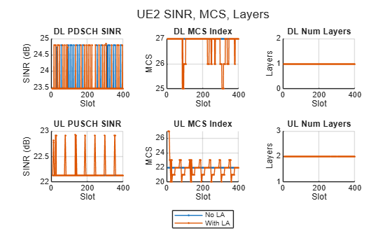
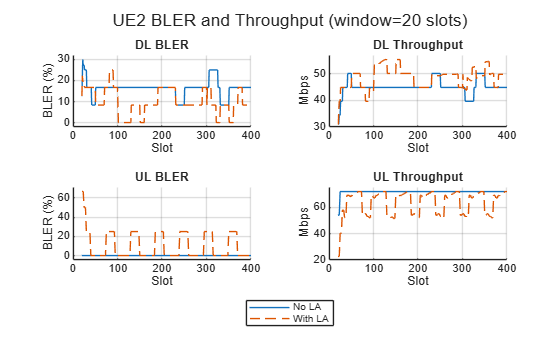
UE2 DL: The large SINR gap (tens of dB) requires many step-down adjustments before the MCS is low enough to result in decodable transport blocks.
UE2 UL: Without OLLA, the MCS selection resulted in a low BLER. With OLLA enabled, the algorithm continuously updates the MCS to achieve a ~10% target. The overall throughput decreases because the marginal MCS increase does not compensate for the retransmission overhead.
This last case illustrates a property of fixed-target OLLA. It is a mechanism that drives all links toward the same BLER target regardless of their starting point. It fixes over-aggressive MCS selection (lowering BLER from 50% to 10%), but it also pushes up link BLERs that were already performing well. For links where the reference signal SINR accurately reflects the data SINR, OLLA provides no benefit and can degrade performance.
References
[1] The OpenStreetMap file is downloaded from https://www.openstreetmap.org, which provides access to crowd-sourced map data all over the world. The data is licensed under the Open Data Commons Open Database License (ODbL), https://opendatacommons.org/licenses/odbl/.
Local Functions
function [logTables,ueInfo,kpiManager] = runNetworkSimulation(networkSimulator, simulationTime, ...
    gnbs, ues, rtChanReg, d, enableLA)
% Run a network simulation using pre-computed ray tracing results

    numgNBs = numel(gnbs);

    % Scheduler configuration
    if enableLA
        laConfig = struct(StepUp=1.8, StepDown=0.2, InitialOffset=-5, ResetOffsetOnCSIReport=false);
        configureScheduler(gnbs, Scheduler="RoundRobin", ...
            CSIMeasurementSignalDL="CSI-RS", ...
            LinkAdaptationConfigUL=laConfig, LinkAdaptationConfigDL=laConfig);
    else
        configureScheduler(gnbs, Scheduler="RoundRobin", ...
            CSIMeasurementSignalDL="CSI-RS");
    end

    addNodes(networkSimulator,gnbs)
    addNodes(networkSimulator,ues)

    % Connect UEs to closest gNB
    [~,idxgnb] = min(d,[],2);
    for n = 1:numgNBs
        connectedUEs = find(idxgnb == n);
        if ~isempty(connectedUEs)
            connectUE(gnbs(n),ues(connectedUEs),FullBufferTraffic="on");
        end
    end

    % Build UE info table: maps UE labels to gNB index, RNTI, and position
    % within the gNB's UE list (used to index into ulUELogs/dlUELogs)
    ueInfoLabel = string.empty; ueInfoGNBIdx = []; ueInfoRNTI = []; ueInfoIdxInGNB = [];
    for n = 1:numgNBs
        uesGNB = ues(ismember([ues.ID],[gnbs(n).UENodeIDs]));
        if ~isempty(uesGNB)
            disp("  "+gnbs(n).Name+": serves "+strjoin([uesGNB.Name],", "))
            for k = 1:numel(uesGNB)
                ueInfoLabel(end+1) = string(uesGNB(k).Name); %#ok<AGROW>
                ueInfoGNBIdx(end+1) = n; %#ok<AGROW>
                ueInfoRNTI(end+1) = uesGNB(k).RNTI; %#ok<AGROW>
                ueInfoIdxInGNB(end+1) = k; %#ok<AGROW>
            end
        end
    end
    ueInfo = table(ueInfoLabel(:), ueInfoGNBIdx(:), ueInfoRNTI(:), ueInfoIdxInGNB(:), ...
        VariableNames=["Label","gNBIdx","RNTI","IdxInGNB"]);

    % Channel model
    addChannelModel(networkSimulator,@rtChanReg.applyChannel);

    % Logging
    numFrames = simulationTime/10e-3;
    metricsVisualizer = cell(numgNBs,1);
    loggers = cell(numgNBs,1);
    for n = 1:numgNBs
        uesGNB = ues(ismember([ues.ID],[gnbs(n).UENodeIDs]));
        if ~isempty(uesGNB)
            metricsVisualizer{n} = helperNRMetricsVisualizer(gnbs(n),uesGNB, ...
                PlotSchedulerMetrics=false,PlotPhyMetrics=false);
            loggers{n} = helperNRSchedulingLogger(numFrames,gnbs(n),uesGNB);
        end
    end

    % KPI manager
    waveformInfo = nrOFDMInfo(gnbs(1).NumResourceBlocks,gnbs(1).SubcarrierSpacing/1e3);
    slotDuration = 1e-3 / waveformInfo.SlotsPerSubframe;  % 0.5 ms for 30 kHz SCS
    kpiManager = hNRKPIManager(KPIString=["phy-bler" "mac-throughput"], ...
        Node={gnbs, ues}, LogInterval=slotDuration);

    % Run simulation
    run(networkSimulator,simulationTime);

    % Collect log tables
    logTables = cell(numgNBs,1);
    for n = 1:numgNBs
        if ~isempty(loggers{n})
            uesGNB = ues(ismember([ues.ID],[gnbs(n).UENodeIDs]));
            logTables{n} = getSimulationLogsTables(loggers{n},gnbs(n).DuplexMode,[uesGNB.RNTI]);
        end
    end
end

function orientations = arrayAnglesToOrientation(arrayAngles)
% Convert array broadside angles [azimuth elevation] (deg), one row per
% node, to node array orientations [azimuth; downtilt; slant] (deg), one
% column per node. Downtilt is the negative of elevation.
    numNodes = size(arrayAngles,1);
    orientations = [arrayAngles(:,1) -arrayAngles(:,2) zeros(numNodes,1)].';
end

function rtChanReg = createChannelRegistry(NRB,SCS,gnbs,ues, ...
    raysDL,raysUL,gnbSites,ueSites,txueUL,rxgNBUL)
% Create the channel registry and add a ray tracing channel for each gNB-UE
% pair. Skip channel creation if no rays exist between the gNB and the UE.

    % Channel model
    numgNBs = numel(gnbs);
    numUEs = numel(ues);
    waveformInfo = nrOFDMInfo(NRB,SCS);
    sr = waveformInfo.SampleRate;
    rtChanReg = RayTracingChannelRegistry([gnbs.ID ues.ID],sr,false);
    for gNBIdx = 1:numgNBs
        for ueIdx = 1:numUEs
            if ~isempty(raysDL{gNBIdx}{ueIdx})
                rtChanReg.addRayTracingChannel(raysDL{gNBIdx}{ueIdx},gnbSites(gNBIdx),ueSites(ueIdx),gnbs(gNBIdx).ID,ues(ueIdx).ID);
            end
            if ~isempty(raysUL{gNBIdx}{ueIdx})
                rtChanReg.addRayTracingChannel(raysUL{gNBIdx}{ueIdx},txueUL(ueIdx),rxgNBUL(gNBIdx),ues(ueIdx).ID,gnbs(gNBIdx).ID);
            end
        end
    end

end

function plotRefVsDataSINR(logTables,ueInfo,wInfo)
    % Plot reference signal SINR vs data channel SINR per slot for each UE

    slotsPerFrame = wInfo.SlotsPerFrame;
    allAxes = gobjects(0);   % array of graphic objects
    for k = 1:height(ueInfo)
        m = ueInfo.gNBIdx(k);
        schLog = logTables{m}.schedulingLogTable;

        figure; tl = tiledlayout(1,2);

        % DL: ref signal SINR vs PDSCH SINR
        dlRows = schLog(strcmp(schLog.Type,'DL') & strcmp(schLog.("Tx Type"),'newTx'), :);
        dlAxes = nexttile(tl,1);
        if ~isempty(dlRows)
            dlSlot = double(dlRows.Frame)*slotsPerFrame+double(dlRows.Slot);
            [dlSlot, dlSortIdx] = sort(dlSlot);
            dlRefSINR = cellfun(@(c) c.SINR, dlRows.("Channel Quality"));
            dlRefSINR = dlRefSINR(dlSortIdx);
            dlDataSINR = dlRows.("SINR (dB)")(dlSortIdx);
            plot(dlSlot, dlRefSINR, '.-'); hold on;
            plot(dlSlot, dlDataSINR, '.-');
            allAxes(end+1) = dlAxes;
        end
        title("DL: Ref Signal vs Data SINR"); ylabel("SINR (dB)"); xlabel("Slot"); grid on;

        % UL: SRS SINR vs PUSCH SINR
        ulRows = schLog(strcmp(schLog.Type,'UL') & strcmp(schLog.("Tx Type"),'newTx'), :);
        ulAxes = nexttile(tl,2);
        if ~isempty(ulRows)
            ulSlot = double(ulRows.Frame)*slotsPerFrame+double(ulRows.Slot);
            [ulSlot, ulSortIdx] = sort(ulSlot);
            ulRefSINR = cellfun(@(c) c.SINR, ulRows.("Channel Quality"));
            ulRefSINR = ulRefSINR(ulSortIdx);
            ulDataSINR = ulRows.("SINR (dB)")(ulSortIdx);
            plot(ulSlot, ulRefSINR, '.-'); hold on;
            plot(ulSlot, ulDataSINR, '.-');
            allAxes(end+1) = ulAxes;
        end
        title("UL: Ref Signal vs Data SINR"); ylabel("SINR (dB)"); xlabel("Slot"); grid on;

        leg = legend(nexttile(tl,1), "Ref Signal SINR","Data SINR");
        leg.Layout.Tile = 'south';
        sgtitle(ueInfo.Label(k) + " SINR Mismatch")
    end
    if ~isempty(allAxes)
        linkaxes(allAxes,'y');
    end
end

function kpis = getBLERandThroughput(kpiManager,simulationTime,slotDuration,windowSize,gnbOfInterest,ueOfInterest)
% Compute windowed DL/UL BLER and throughput over the simulation duration

    % Number of slots in simulation
    numSlots = round(simulationTime / slotDuration);

    % Skip first (windowSize-1) slots where the backward-looking window is partial
    numSlotsInPlot = numSlots-windowSize+1;
    dlBLER = zeros(1, numSlotsInPlot);
    ulBLER = zeros(1, numSlotsInPlot);
    dlThput = zeros(1, numSlotsInPlot);
    ulThput = zeros(1, numSlotsInPlot);

    windowDuration = windowSize*slotDuration;
    for idx = 1:numSlotsInPlot
        % Current time at the end of this slot
        currentTime = (idx+windowSize-1)*slotDuration;

        % Windowed BLER: [currentTime - windowDuration, currentTime]
        windowStart = currentTime-windowDuration;
        windowEnd = currentTime;

        dlBLER(idx) = kpi(kpiManager, (gnbOfInterest), (ueOfInterest), "phy-bler", ...
            StartTime=windowStart, EndTime=windowEnd, LinkType="DL")*100;

        ulBLER(idx) = kpi(kpiManager, (ueOfInterest), (gnbOfInterest), "phy-bler", ...
            StartTime=windowStart, EndTime=windowEnd, LinkType="UL")*100;

        % Windowed throughput: [currentTime - windowDuration, currentTime]
        dlThput(idx) = kpi(kpiManager, (gnbOfInterest), (ueOfInterest), "mac-throughput", ...
            StartTime=windowStart, EndTime=windowEnd, LinkType="DL");

        ulThput(idx) = kpi(kpiManager, (ueOfInterest), (gnbOfInterest), "mac-throughput", ...
            StartTime=windowStart, EndTime=windowEnd, LinkType="UL");
    end

    kpis = struct();
    kpis.dlBLER = dlBLER;
    kpis.ulBLER = ulBLER;
    kpis.dlThput = dlThput;
    kpis.ulThput = ulThput;
    kpis.kpiSlotRange = windowSize:numSlots;  % X-axis shows actual slot numbers

end

function tl = plotKPIs(kpiSlotRange,dlBLER,dlThput,ulBLER,ulThput,legendLabels)
% Plot DL/UL BLER and throughput

    figure; tl = tiledlayout(2,2);

    data = {dlBLER, dlThput, ulBLER, ulThput};
    titles = ["DL BLER", "DL Throughput", "UL BLER", "UL Throughput"];
    ylabels = ["BLER (%)", "Mbps", "BLER (%)", "Mbps"];

    for t = 1:4
        nexttile(tl,t);
        hold on;
        lineStyles = ["-", "--"];
        for r = 1:size(data{t},1)
            plot(kpiSlotRange, data{t}(r,:), lineStyles(r));
        end
        xlabel("Slot")
        ylabel(ylabels(t));
        title(titles(t));
        grid on;
        ylim padded
    end

    if nargin >= 6
        leg = legend(nexttile(tl,1), legendLabels);
        leg.Layout.Tile = 'south';
    end
end

function plotSINRandMCS(logTablesIn, ueInfo, wInfo, legendLabels)
    % Plot per-UE SINR, MCS, and layers (2x3 tiled figure).
    %   logTablesIn: a single logTables cell array, or a cell array of
    %                logTables (one per simulation run).
    %   ueInfo:      table with columns Label, gNBIdx, RNTI, IdxInGNB.
    %   wInfo:       nrOFDMInfo output.
    %   legendLabels (optional): string array with one label per run.

    % Normalize input: wrap a single logTables in a cell
    if ~iscell(logTablesIn{1})
        allLogs = {logTablesIn};
    else
        allLogs = logTablesIn;
    end

    slotsPerFrame = wInfo.SlotsPerFrame;
    metrics = ["SINR (dB)", "MCS Index", "NumLayers"];
    titlesDL = ["DL PDSCH SINR", "DL MCS Index", "DL Num Layers"];
    titlesUL = ["UL PUSCH SINR", "UL MCS Index", "UL Num Layers"];
    yLabels = ["SINR (dB)", "MCS", "Layers"];

    for u = 1:height(ueInfo)
        m = ueInfo.gNBIdx(u);
        idx = ueInfo.IdxInGNB(u);
        ueLabel = ueInfo.Label(u);

        figure; tl = tiledlayout(2,3);

        for s = 1:numel(allLogs)
            dlLog = allLogs{s}{m}.dlUELogs{idx};
            ulLog = allLogs{s}{m}.ulUELogs{idx};

            slotDL = dlLog.Frame.*slotsPerFrame+dlLog.Slot;
            [slotDL, sortDL] = sort(slotDL);
            slotUL = ulLog.Frame.*slotsPerFrame+ulLog.Slot;
            [slotUL, sortUL] = sort(slotUL);

            for col = 1:3
                nexttile(tl, col); hold on; grid on;
                plot(slotDL, dlLog.(metrics(col))(sortDL), '.-');
                title(titlesDL(col)); ylabel(yLabels(col)); xlabel("Slot");

                nexttile(tl, col+3); hold on; grid on;
                plot(slotUL, ulLog.(metrics(col))(sortUL), '.-');
                title(titlesUL(col)); ylabel(yLabels(col)); xlabel("Slot");
            end
        end

        if nargin >= 4 && ~isempty(legendLabels)
            leg = legend(nexttile(tl,1), legendLabels);
            leg.Layout.Tile = 'south';
        end
        sgtitle(ueLabel + " SINR, MCS, Layers")
    end
end

function cartCoordinates = latLonToCartesianFlatEarth(latLon,totalAntennaHeight,latLonReference)
% Cartesian (flat-Earth) approximation using an equirectangular projection
% about a reference latitude and longitude. Accurate to sub-meter level for
% areas up to a few kilometers.

    metersPerDeg = 111319.5; % 2piR/360, with R the Earth radius at the equator
    x = (latLon(2)-latLonReference(2))*cosd(latLonReference(1))*metersPerDeg; % East
    y = (latLon(1)-latLonReference(1))*metersPerDeg;                            % North
    z = totalAntennaHeight;                                                         % Up
    cartCoordinates = [x,y,z];
end

function validategNBArraySize(arraySize)
% Validate arraySize ([rows columns]) array size.
%  [1 1]
%  [1 2]
%  [2 2]
%  [2 4]
%  [4 4]

    validSizes = [1 1;
        1 2;
        2 2;
        2 4;
        4 4];

    % Check arraySize validity
    if ~ismember(arraySize(:).',validSizes,"rows")
        error("Invalid gNB array size ("+mat2str(arraySize)+"). Valid sizes are: "+mat2str(validSizes))
    end
end

function BW = validateNumerology(SCS,NRB)
% Validate subcarrier spacing and grid size values and return the bandwidth in Hz

    % Channel transmission bandwidth configuration table (SCS, BW and NRB)
    txBwConfig = nrDLCarrierConfig.FR1BandwidthTable;
    rowName = string(SCS+"kHz"); % SCS to string

    % Validate SCS
    if ~ismember(rowName, string(txBwConfig.Properties.RowNames))
        error("Invalid SCS ("+SCS+"). Value must be a member of: "+ ...
            strjoin(erase(string(txBwConfig.Properties.RowNames),"kHz")));
    end

    nrbRow = txBwConfig{rowName, :};             % Extract the row of NRB values
    validMask = ~isnan(nrbRow);                   % Valid entries are those that are not NaN
    matchMask = validMask & (nrbRow == NRB);      % Find exact NRB matches among valid entries
    if any(matchMask)
        % Column names where there is a match
        bwVars = string(txBwConfig.Properties.VariableNames(matchMask));
        % Convert "XXMHz" to numeric Hz
        BW = str2double(erase(bwVars, "MHz"))*1e6; % Remove the "MHz" suffix and convert to double
    else
        disp("Valid channel transmission bandwidth configurations: SCS, bandwidth and NRBs.")
        disp(txBwConfig)
        [~,idx]=min(abs(nrbRow-NRB));
        error("Invalid combination of SCS ("+SCS+" kHz) and NRB ("+NRB+"). "+newline+ ...
            "Select a valid combination from the channel transmission bandwidth configuration table."+newline+ ...
            "The closest set of values in the table is SCS = "+SCS+"kHz, and NRB = "+nrbRow(idx));
    end
end

function [dlFc,ulFc] = fddCarrierFreq(duplexingMode,fc,channelBandwidth)
% Return the downlink and uplink channels center carrier frequency

    if duplexingMode=="TDD"
        dlFc = fc;
        ulFc = fc;
    else
        % DL/UL band offset is  +/- guardBand*0.5 Hz of the carrier frequency and is
        % channelBandwidth Hz wide.
        guardBand = 140e6;
        dlFc = fc+guardBand/2+channelBandwidth/2;
        ulFc = fc-guardBand/2-channelBandwidth/2;
    end
end

function raysUL = dl2ulRays(rays)
% Convert downlink rays to uplink rays when we assume channel reciprocity.
% This function swaps the transmitter and receiver locations, "flips" the
% interaction matrix, and transposes the polarization matrix. Other uplink
% ray properties remain the same. Constructing the uplink rays this way
% results in the swapping of the angles of arrival and departure.
    raysUL = rays;
    for n = 1:numel(rays)
        for m = 1:numel(rays{n})
            raysUL{n}(m).TransmitterLocation = rays{n}(m).ReceiverLocation;
            raysUL{n}(m).ReceiverLocation = rays{n}(m).TransmitterLocation;
            raysUL{n}(m).PolarizationMatrix = rays{n}(m).PolarizationMatrix.';
            raysUL{n}(m).Interactions = flip(rays{n}(m).Interactions);
        end
    end
end

function [txUL,rxUL] = createULSites(tx,rx,PtxUEW,ulFc)
% Turn tx sites into rxsites. This is used to perform ray tracing in the
% uplink
    ngNBs = numel(tx);
    rxUL = rxsite.empty();
    for n = ngNBs:-1:1
        rxArrayUL = tx(n).Antenna.clone();
        rxUL(n) = rxsite(Latitude=tx(n).Latitude,Longitude=tx(n).Longitude, ...
            Antenna=rxArrayUL,AntennaAngle=tx(n).AntennaAngle, ...
            AntennaHeight=tx(n).AntennaHeight);
    end
    nUEs = numel(rx);
    txUL = txsite.empty();
    for n = nUEs:-1:1
        txArrayUL = rx(n).Antenna.clone();
        txUL(n) = txsite(Latitude=rx(n).Latitude,Longitude=rx(n).Longitude, ...
            TransmitterPower=PtxUEW,TransmitterFrequency=ulFc, ...
            Antenna=txArrayUL,AntennaHeight=rx(n).AntennaHeight, ...
            AntennaAngle=rx(n).AntennaAngle);
    end
end

