Miniaturize Microstrip Patch Antenna Using Slot-Loading and Genetic Algorithm Optimization

Define Antenna Parameters

The antenna design starts with a square microstrip patch on an air substrate. This example uses Air ($${ϵ}_r=1$$) as the dielectric to simplify fabrication and eliminate dielectric loss, though it requires a larger patch for a given frequency compared to higher-permittivity substrates. The 100 mm square ground plane provides enough extent (approximately $$0.9\lambda$$ at the resonant frequency) to minimize edge diffraction effects on the radiation pattern. The 53 mm patch dimension places the fundamental $${\text{TM}}_{010}$$ mode resonance near 2.6 GHz.

height = 4.3e-3;
substrate = dielectric("Air");
substrate.Thickness = height;

groundPlaneLength = 100e-3;
groundPlaneWidth = 100e-3;

patchLength = 53e-3;
patchWidth = 53e-3;

feedLocation = [-7.5e-3, -3.64e-3, height];

Create and Analyze Square Patch Antenna

Build the baseline square patch antenna using a pcbStack object with three layers: the conducting patch on top, an air substrate in the middle, and a conducting ground plane on the bottom. The feed is a probe (coaxial pin) offset from center. The feed position used here is optimized for the H-patch variant (which is the primary design of interest); for the square patch it provides a reference for the resonance frequency but might not achieve ideal 50 $$\Omega$$ matching. In practice, adjust the feed position for each variant independently.

ground = antenna.Rectangle(Length=groundPlaneLength, Width=groundPlaneWidth, Center=[0 0]);
patchRect = antenna.Rectangle(Length=patchLength, Width=patchWidth, Center=[0 0]);

squarePatchAnt = pcbStack;
squarePatchAnt.BoardThickness = height;
squarePatchAnt.BoardShape = ground;
squarePatchAnt.Layers = {patchRect, substrate, ground};
squarePatchAnt.FeedLocations = [feedLocation(1:2), 1, 3];

figure
show(squarePatchAnt)
title("Square Patch Antenna")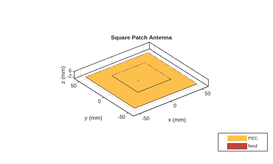

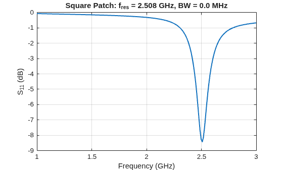
Compute the return loss ($$S_{11}$$) over a wide frequency range spanning 1 to 3 GHz. This range is broad enough to capture the fundamental resonance and any higher-order modes that might appear.

freqRange = linspace(1e9, 3e9, 200);
S_square = sparameters(squarePatchAnt, freqRange);
S11_square = 20*log10(abs(rfparam(S_square, 1, 1)));

[minS11_square, idx] = min(S11_square);
fres_square = freqRange(idx);
bw_square = computeBandwidth(S11_square, freqRange);

figure
plot(freqRange/1e9, S11_square, "LineWidth", 1.5)
grid on
xlabel("Frequency (GHz)")
ylabel("S_{11} (dB)")
title(sprintf("Square Patch: f_{res} = %.3f GHz, BW = %.1f MHz", ...
    fres_square/1e9, bw_square/1e6))

Compute the realized gain pattern at the resonance frequency. The realized gain includes mismatch loss and gives the most practically relevant measure of antenna performance.

[gainData_square, ~, ~] = pattern(squarePatchAnt, fres_square, Type="realizedgain");
peakGain_square = max(gainData_square(:));

figure
pattern(squarePatchAnt, fres_square, Type="realizedgain")
title(sprintf("Square Patch: Realized Gain at %.2f GHz", fres_square/1e9))

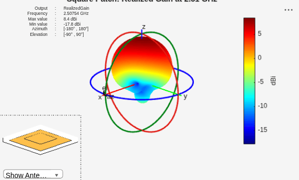
The square patch resonates near 2.5 GHz with a broadside radiation pattern characteristic of the fundamental $${\text{TM}}_{010}$$ mode. The matching is not optimal at this feed location (tuned for the H-patch), but the resonance frequency establishes the baseline. The key observation is that this 53 mm patch resonates near 2.5 GHz. Slot-loading shifts this significantly lower without changing the footprint.

Create Slot-Loaded H-Patch Antenna

Miniaturize the patch by subtracting two symmetric rectangular notches from opposite edges, creating an H-shaped geometry. The notches interrupt the direct current path between the radiating edges, forcing the surface current to detour around the slots. This longer meandering path increases the effective electrical length of the resonator without increasing its physical footprint, thereby reducing the resonance frequency.

This example sets the notch dimensions (15.3 mm long by 3.51 mm wide) to produce a significant frequency shift while keeping the antenna well-matched. Deeper notches produce more miniaturization but eventually compromise radiation efficiency and bandwidth.

notchLength = 15.3e-3;
notchWidth = 3.51e-3;
notchCenter = [patchLength/2 - notchLength/2, 0];

notch1 = antenna.Rectangle(Length=notchLength, Width=notchWidth, Center=notchCenter);
notch2 = antenna.Rectangle(Length=notchLength, Width=notchWidth, Center=-notchCenter);

hPatch = patchRect - notch1 - notch2;

hPatchAnt = pcbStack;
hPatchAnt.BoardThickness = height;
hPatchAnt.BoardShape = ground;
hPatchAnt.Layers = {hPatch, substrate, ground};
hPatchAnt.FeedLocations = [feedLocation(1:2), 1, 3];

figure
show(hPatchAnt)
title("H-Patch Antenna (Slot-Loaded)")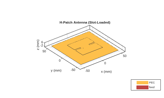

Compute the S-parameters and gain for the H-patch to quantify the effect of slot-loading.

S_hpatch = sparameters(hPatchAnt, freqRange);
S11_hpatch = 20*log10(abs(rfparam(S_hpatch, 1, 1)));

[minS11_hpatch, idx] = min(S11_hpatch);
fres_hpatch = freqRange(idx);
bw_hpatch = computeBandwidth(S11_hpatch, freqRange);

[gainData_hpatch, ~, ~] = pattern(hPatchAnt, fres_hpatch, Type="realizedgain");
peakGain_hpatch = max(gainData_hpatch(:));

Plot the return loss of both antennas on the same axes to visualize the frequency shift achieved by slot-loading.

figure
plot(freqRange/1e9, S11_square, "LineWidth", 1.5, "DisplayName", ...
    sprintf("Square Patch (f_r = %.2f GHz)", fres_square/1e9))
hold on
plot(freqRange/1e9, S11_hpatch, "LineWidth", 1.5, "DisplayName", ...
    sprintf("H-Patch (f_r = %.2f GHz, BW = %.0f MHz)", fres_hpatch/1e9, bw_hpatch/1e6))
yline(-10, "--k", "DisplayName", "-10 dB Threshold")
hold off
grid on
xlabel("Frequency (GHz)")
ylabel("S_{11} (dB)")
legend("Location", "best")
title("Effect of Slot-Loading on Resonance Frequency")

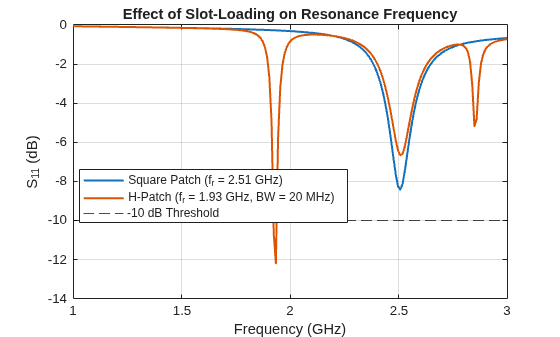
The slot-loading shifts the resonance from approximately 2.5 GHz down to about 1.9 GHz — a reduction of roughly 23% — without changing the antenna footprint. This is equivalent to making the antenna electrically smaller by nearly a quarter wavelength. The H-patch achieves good matching ($$S_{11}<-10$$ dB) with a bandwidth of approximately 20 MHz. This bandwidth-miniaturization tradeoff is fundamental: a smaller electrical aperture stores more reactive energy relative to radiated power, which narrows the bandwidth according to the Chu-Harrington limit.

The next sections show how to use a Genetic Algorithm to either push the miniaturization further (at the expense of more bandwidth) or recover some of the lost bandwidth while retaining a compact footprint.

Set Up Pixelation Grid for Optimization

To enable automated shape optimization, divide one quadrant of the H-patch into a grid of small rectangular pixels. Each pixel represents a binary design variable: 1 means metal is present, 0 means metal is removed (a slot is cut). The GA searches through combinations of these binary variables to find geometries that optimize a chosen performance metric.

The grid covers only one quadrant because the design mirrors the pattern across both the $$x$$-axis and $$y$$-axis to enforce four-fold symmetry. This symmetry constraint serves two purposes: it preserves a clean, symmetric radiation pattern with predictable polarization, and it reduces the effective design space from $$24\times 24=576$$ variables down to $$12\times 12=144$$ variables, making the optimization tractable.

Additionally, the optimization always keeps the outermost row and column of pixels metallic (value = 1) to maintain the structural perimeter of the patch, and always protects the region around the feed probe to ensure a continuous current path to the excitation point.

nx = 12;
ny = 12;

unitPatchWidth = patchWidth/2/ny;
unitPatchLength = patchLength/2/nx;
overlapWidth = unitPatchWidth * 0.1;

unitPatches = cell(nx, ny);
for i = 1:nx
    for j = 1:ny
        unitPatches{i,j} = antenna.Rectangle( ...
            Length=unitPatchLength + overlapWidth/2, ...
            Width=unitPatchWidth + overlapWidth/2, ...
            Center=[(i-1)*unitPatchLength + unitPatchLength/2, ...
                    (j-1)*unitPatchWidth + unitPatchWidth/2]);
    end
end

Each pixel in the 12$$\times$$12 grid measures approximately 2.2 mm $$\times$$ 2.2 mm. With the four-fold mirror symmetry, the effective resolution is 24$$\times$$24 pixels across the full 53 mm patch, giving a spatial resolution of about $$\lambda /60$$ at 2 GHz. The 10% overlap between adjacent pixels helps ensure that the resulting geometry remains a connected conductor even after pixels are removed. Without this overlap, diagonal removals could create isolated metal islands that would not participate in radiation.

Define Optimization Cost Functions

Two cost functions target different engineering objectives that a designer might face in practice.

Cost 1 — Miniaturization (frequency reduction):

This multi-objective cost function primarily rewards lower resonance frequency (first term). The second term penalizes poor return loss. Without it, the optimizer might find geometries that resonate at very low frequencies but cannot be excited efficiently. The third term rewards higher gain to avoid degenerate solutions where most of the patch has been removed and the antenna no longer radiates effectively. This example selects the weighting coefficients (10, 0.1, 0.2) empirically to balance these objectives so that frequency reduction dominates while maintaining practical performance.

Cost 2 — Bandwidth enhancement:

This cost function simply maximizes the $$-$$10 dB impedance bandwidth in MHz. The negative sign converts the maximization problem into a minimization for compatibility with the GA solver. During bandwidth optimization, the frequency sweep range is set to 1.8–2.3 GHz, allowing the resonance to shift upward from the H-patch frequency but constraining it below the original square patch resonance.

Configure Genetic Algorithm

The Genetic Algorithm from the Optimization Toolbox evolves a population of candidate designs through selection, crossover, and mutation. Each individual in the population is a 144-element binary vector representing the pixel states for one quadrant. The GA uses integer constraints to ensure all variables are exactly 0 or 1.

At each generation, every candidate is evaluated by: constructing the modified patch geometry, building a PCB antenna, computing S-parameters with the Method of Moments solver, finding the resonance frequency, computing the realized gain pattern, and evaluating the cost function. This makes each function evaluation computationally expensive (several seconds), so the population size and number of generations must balance solution quality against runtime.

options = optimoptions("ga", ...
    UseParallel=false, ...
    PlotFcn="gaplotbestf", ...
    ConstraintTolerance=1e-3, ...
    MaxGenerations=10, ...
    CrossoverFraction=0.9, ...
    EliteCount=1, ...
    PopulationSize=10);

With |PopulationSize=10| and |MaxGenerations=10|, this configuration evaluates approximately 100 candidate antennas and runs in 10–20 minutes on a typical workstation. For production-quality results, increase |PopulationSize| to 30–50 and |MaxGenerations| to 50–100 (requiring several hours of computation). Setting |UseParallel=true| with the Parallel Computing Toolbox distributes evaluations across CPU cores for near-linear speedup.

The GA call takes this form:

 [x, fval] = ga(@(v) objectiveFunction(inputs, v), ...
        nx*ny, [], [], [], [], ...
        zeros(1, nxny), ones(1, nxny), [], ...
        1:nx*ny, options);

The integer constraint (argument before |options|) ensures all 144 pixel values are exactly 0 or 1. The lower bound is all zeros (maximum metal removal) and the upper bound is all ones (solid patch). The edge-forcing and feed protection happen inside the objective function, not through the bounds.

How Objective Function Works

Inside the objective function, the GA candidate vector is transformed into a physical antenna through these steps:

The four-fold mirroring in step 3 is the key insight: by optimizing only 144 variables instead of 576, the search space is reduced by a factor of 4 while guaranteeing symmetric radiation patterns. This makes the GA converge in a practical number of generations.

Examine Miniaturization Results

Load pre-computed GA results from a miniaturization optimization run. The optimizer explored many candidate geometries over multiple generations, evaluating each one by building the antenna, computing S-parameters, and calculating the multi-objective cost function (Cost 1). The optimization saves all intermediate results including patch geometries, S-parameters, resonance frequencies, bandwidth, and gain for post-processing.

ResultsFreq = load("Results_test_freq.mat");
ResultsFreq = ResultsFreq.Results;

Extract the performance metrics from the saved results. Each row in the cost data corresponds to one candidate antenna evaluated during the GA run.

range = ResultsFreq.range;
costData = ResultsFreq.Costvalues;
S11data = ResultsFreq.S11';

s11min = costData(:,3);
gain = costData(:,4);
fres = costData(:,5);
bw = costData(:,6)/1e6;

Filter for candidate antennas that simultaneously achieve meaningful miniaturization (resonance below 1.6 GHz), adequate impedance matching ($$S_{11}<-10$$ dB), useful gain (above 7 dBi), and some measurable bandwidth (above 3 MHz). These thresholds represent the minimum requirements a designer would typically accept for a practical miniaturized antenna.

candidates = find(s11min < -10 & fres < 1.6 & gain > 7 & bw > 3);
numTotal = size(costData, 1);
numPassing = numel(candidates);

Display the best miniaturized antenna geometry. The GA removed interior pixels in a pattern that creates additional current meandering paths beyond what the two notches alone provide, further reducing the resonance frequency.

if ~isempty(candidates)
    [~, bestIdx] = min(fres(candidates));
    bestCase = candidates(bestIdx);

    figure
    show(ResultsFreq.patchNew(bestCase))
    title(sprintf("Optimized Patch (Miniaturization): f_{res} = %.2f GHz", fres(bestCase)))
    axis off
end

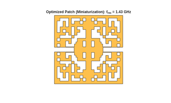
Compare the S-parameters of the square patch, H-patch, and GA-optimized patch on the same axes. The progressive shift of the resonance to lower frequencies shows the cumulative effect of slot-loading (H-patch notches) followed by interior pixelation (GA optimization).

if ~isempty(candidates)
    figure
    plot(freqRange/1e9, S11_square, "LineWidth", 1.5, "DisplayName", ...
        sprintf("Square Patch (%.2f GHz)", fres_square/1e9))
    hold on
    plot(freqRange/1e9, S11_hpatch, "LineWidth", 1.5, "DisplayName", ...
        sprintf("H-Patch (%.2f GHz)", fres_hpatch/1e9))
    plot(range/1e9, S11data(bestCase,:), "LineWidth", 1.5, "DisplayName", ...
        sprintf("GA Optimized (%.2f GHz)", fres(bestCase)))
    yline(-10, "--k", "HandleVisibility", "off")
    hold off
    grid on
    xlabel("Frequency (GHz)")
    ylabel("S_{11} (dB)")
    legend("Location", "best")
    title("Miniaturization Progression: S_{11} Comparison")
end

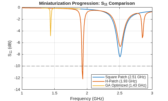
The GA-optimized design achieves a resonance near 1.4 GHz representing a 43% frequency reduction from the original square patch and a further 26% below the H-patch alone. This means the antenna is electrically 43% smaller at its operating frequency. The tradeoff is a narrower impedance bandwidth (approximately 3 MHz), which is expected when pushing miniaturization toward fundamental limits. For narrowband applications such as sensor networks, RFID, or telemetry links, this bandwidth is often acceptable.

Compute and display the radiation pattern of the optimized miniaturized antenna to verify that the gain remains usable despite the aggressive miniaturization.

if ~isempty(candidates)
    antOpt = buildOptimizedAntenna(ResultsFreq.patchNew(bestCase), ...
        height, substrate, ground, feedLocation);
    figure
    pattern(antOpt, fres(bestCase)*1e9, Type="realizedgain")
    title(sprintf("Miniaturized Antenna: Realized Gain at %.2f GHz", fres(bestCase)))
end

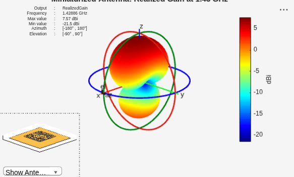
The radiation pattern retains the broadside characteristic of a patch antenna, confirming that the pixelation has not introduced undesirable pattern distortion. The realized gain remains above 7 dBi, which is only about 1 dB below the original square patch despite the 40% frequency reduction.

Examine Bandwidth Optimization Results

Load results from a separate optimization run that targeted bandwidth maximization using Cost 2. Here the GA searched for pixel patterns that widen the $$-$$10 dB impedance bandwidth while allowing the resonance to shift in the 1.8–2.3 GHz range. The goal is to recover or exceed the bandwidth lost when you added the notches to form the H-patch.

ResultsBW = load("Results_test_BW.mat");
ResultsBW = ResultsBW.Results;

Extract metrics and filter for candidates with meaningful bandwidth improvement. The threshold of 40 MHz represents approximately double the H-patch bandwidth, confirming the optimization has achieved a significant improvement over the nonoptimized slot-loaded design.

range_bw = ResultsBW.range;
costData_bw = ResultsBW.Costvalues;
S11data_bw = ResultsBW.S11';

fres_bw = costData_bw(:,5);
bw_bw = costData_bw(:,6)/1e6;
s11min_bw = costData_bw(:,3);
gain_bw = costData_bw(:,4);

candidates_bw = find(s11min_bw < -10 & fres_bw < 2.22 & gain_bw > 7 & bw_bw > 40);

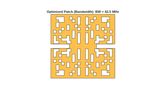
Display the best bandwidth-optimized antenna geometry. Notice how the pixel removal pattern differs from the miniaturization case — here the optimizer creates features that introduce additional closely-spaced resonances, which merge to form a wider passband.

if ~isempty(candidates_bw)
    [~, bestIdx_bw] = max(bw_bw(candidates_bw));
    bestCase_bw = candidates_bw(bestIdx_bw);

    figure
    show(ResultsBW.patchNew(bestCase_bw))
    title(sprintf("Optimized Patch (Bandwidth): BW = %.1f MHz", bw_bw(bestCase_bw)))
    axis off
end

Compare the bandwidth performance across all three antenna variants. The $$-$$10 dB threshold line indicates the frequency band over which the antenna achieves good matching (return loss better than 10 dB, or less than 10% reflected power).

if ~isempty(candidates_bw)
    figure
    plot(freqRange/1e9, S11_square, "LineWidth", 1.5, "DisplayName", ...
        sprintf("Square Patch (f_r = %.2f GHz)", fres_square/1e9))
    hold on
    plot(freqRange/1e9, S11_hpatch, "LineWidth", 1.5, "DisplayName", ...
        sprintf("H-Patch (BW = %.0f MHz)", bw_hpatch/1e6))
    plot(range_bw/1e9, S11data_bw(bestCase_bw,:), "LineWidth", 1.5, "DisplayName", ...
        sprintf("GA Optimized (BW = %.0f MHz)", bw_bw(bestCase_bw)))
    yline(-10, "--k", "HandleVisibility", "off")
    hold off
    grid on
    xlabel("Frequency (GHz)")
    ylabel("S_{11} (dB)")
    legend("Location", "best")
    title("Bandwidth Optimization: S_{11} Comparison")
end

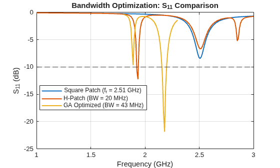
The bandwidth-optimized design recovers significant bandwidth compared to the plain H-patch. With a resonance near 2.2 GHz, the optimized patch achieves over 40 MHz of bandwidth — more than double the H-patch's 20 MHz — while maintaining a form factor that is still more compact than the original square patch. The gain remains above 7 dBi, confirming that the internal pixel removal has not degraded radiation efficiency. This result shows that judicious geometry optimization can partially overcome the fundamental bandwidth-miniaturization tradeoff.

Summary of Results

The table below compares all four antenna variants side by side. The progression from square patch through H-patch to the two optimized designs illustrates the design trade-space available through slot-loading and pixelated optimization.

variantNames = ["Square Patch*"; "H-Patch (Slot-Loaded)"; ...
    "GA Optimized (Miniaturization)"; "GA Optimized (Bandwidth)"];
freqValues = [fres_square/1e9; fres_hpatch/1e9; fres(bestCase); fres_bw(bestCase_bw)];
bwValues = [NaN; bw_hpatch/1e6; bw(bestCase); bw_bw(bestCase_bw)];
gainValues = [peakGain_square; peakGain_hpatch; gain(bestCase); gain_bw(bestCase_bw)];

T = table(variantNames, freqValues, bwValues, gainValues, ...
    VariableNames=["Antenna", "Resonance (GHz)", "Bandwidth (MHz)", "Peak Gain (dBi)"])

T = 4×4 table
                Antenna                 Resonance (GHz)    Bandwidth (MHz)    Peak Gain (dBi)
    ________________________________    _______________    _______________    _______________

    "Square Patch*"                         2.5075                NaN             8.3982     
    "H-Patch (Slot-Loaded)"                 1.9347             20.101             7.4542     
    "GA Optimized (Miniaturization)"        1.4289             3.1839             7.5395     
    "GA Optimized (Bandwidth)"               2.178             42.505             8.8009     

*The square patch uses a feed position optimized for the H-patch and is not matched below $$-$$10 dB at this feed location. This table does not report its bandwidth. In practice, moving the feed to approximately $$(0,-10)$$ mm provides a well-matched square patch with ~80 MHz bandwidth at 2.5 GHz.

The results show two distinct optimization strategies for the same antenna platform:

In practice, an engineer can also define hybrid cost functions that balance both objectives simultaneously, or add constraints on cross-polarization, pattern symmetry, or efficiency. The pixel-based GA framework is flexible enough to accommodate any scalar cost function that can be computed from the antenna's electromagnetic response.

Supporting Functions

function bw = computeBandwidth(S11_dB, freqVec)
    [minVal, minIdx] = min(S11_dB);
    if minVal < -10
        below = S11_dB < -10;
        crossings = find(diff(below));
        if numel(crossings) >= 2
            fLow = freqVec(crossings(1));
            fHigh = freqVec(crossings(end));
            bw = fHigh - fLow;
        else
            [~, idx] = mink(abs(S11_dB + 10), 2);
            bw = abs(diff(freqVec(sort(idx))));
        end
    else
        bw = 0;
    end
end

function ant = buildOptimizedAntenna(patchShape, height, substrate, ground, feedLocation)
    ant = pcbStack;
    ant.BoardThickness = height;
    ant.BoardShape = ground;
    ant.Layers = {patchShape, substrate, ground};
    ant.FeedLocations = [feedLocation(1:2), 1, 3];
end

References

[1] H. T. Nguyen, S. Noghanian, and L. Shafai, "Microstrip patch miniaturization by slots loading," 2005 IEEE Antennas and Propagation Society International Symposium, Washington, DC, 2005, pp. 215-218.

[2] H. T. Nguyen, "Miniaturizing microstrip patch antenna by slot-loading," M.Sc. Thesis, University of Manitoba, Winnipeg, Canada, 2006.

[3] A. Sabouni, S. Noghanian, M. S. Abrishamian, and M. M. Zahedi, "Optimization of microstrip patch antenna using Genetic Algorithm method," 11th International Symposium on Antenna Technology and Applied Electromagnetics (ANTEM 2005), Saint-Malo, France, 2005.

[4] S. Noghanian, R. Fazel-Rezai, H. T. Nguyen, A. Sabouni, and L. Shafai, "Microstrip Antenna Miniaturization using Slot-Loading," 2025 IEEE International Symposium on Antennas and Propagation and ITNC-USNC-URSI Radio Science Meeting (AP-S/URSI), Montreal, QC, Canada, 2025.