Miniaturize Rectangular Microstrip Patch Antenna Using Genetic Algorithm Optimization

This example uses:

This example shows how to miniaturize a rectangular microstrip patch antenna by using a genetic algorithm for topology optimization. In this example, you divide the rectangular patch into small equal sized patches. Based on GA optimization values, you remove some patches to reduce the resonance frequency [1,2].

Create Microstrip Patch Antenna at 4.9 GHz

Specify the feed, substrate, ground plane, and patch dimensions. Define the feed location. Create the microstrip patch antenna of size 17.58-by-13.85 mm on FR4 substrate with thickness of 1.6 mm and a stepped microstrip feed to resonate around 4.9 GHz. using pcbStack.

% Stepped feed parameters
inputs.f2Width = 8.34e-3;
inputs.f1Width = 10e-3;
inputs.f2Length = 1.5e-3;
inputs.f1Length = 2.87e-3;

% Substrate parameters
inputs.height = 1.6e-3; 
inputs.Subs = dielectric("FR4");
inputs.Subs.Thickness = inputs.height;

% Ground plane parameters
inputs.groundPlaneLength = 25e-3; 
inputs.groundPlaneWidth = 50e-3;

% Create the feed strip
f1 = antenna.Rectangle(Length=inputs.f1Length, Width=inputs.f1Width, Center=[0, -inputs.groundPlaneWidth/2+inputs.f1Width/2]);
f2 = antenna.Rectangle(Length=inputs.f2Length, Width=inputs.f2Width, Center=[0, -inputs.groundPlaneWidth/2+inputs.f1Width+inputs.f2Width/2]);
inputs.feedArea = f1 + f2;

% Feed location
inputs.feedLocation = [0, -inputs.groundPlaneWidth/2, inputs.height];

% Create the ground plane
inputs.ground = antenna.Rectangle(Length=inputs.groundPlaneLength, Width=inputs.groundPlaneWidth, Center=[0 0]);

% Patch parameters
inputs.patchLength = 17.58e-3;
inputs.patchWidth = 13.85e-3;

patchRect5GHz = antenna.Rectangle(Length=inputs.patchLength, Width=inputs.patchWidth, ...
    Center=[0, -inputs.groundPlaneWidth/2+inputs.f1Width+inputs.f2Width+inputs.patchWidth/2]);

finalPatch5GHz  = inputs.feedArea + patchRect5GHz; 

antAt5GHz = pcbStack(Layers={finalPatch5GHz, inputs.Subs inputs.ground}, BoardThickness=inputs.height, ...
    BoardShape=inputs.ground, FeedLocations=[inputs.feedLocation(1:2), 1, 3]);

figure
show(antAt5GHz);

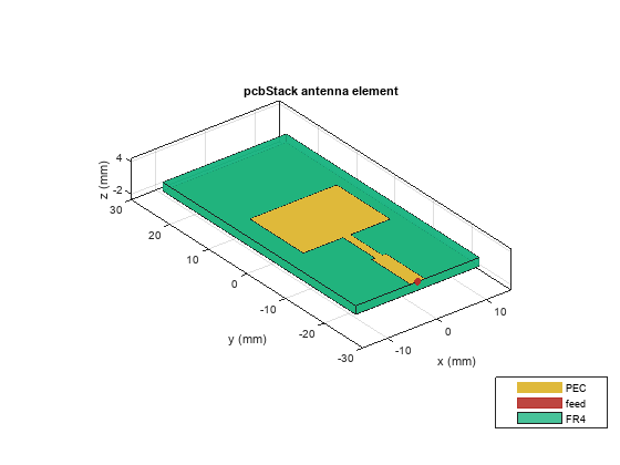
Figure contains an axes object. The axes object with title pcbStack antenna element, xlabel x (mm), ylabel y (mm) contains 6 objects of type patch, surface. These objects represent PEC, feed, FR4.

figure 
rfplot(sparameters(antAt5GHz,linspace(1.5e9,5.5e9,100)));

$Figure contains an axes object. The axes object with xlabel Frequency (GHz), ylabel Magnitude (dB) contains an object of type line. This object represents dB(S_{11}).$

Optimize Antenna Using Genetic Algorithm

Apply the material distributive approach topology optimization by using a genetic algorithm to reduce the resonance frequency of the patch antenna. In GA optimization, you first create an initial population. At each iteration, the algorithm uses the individuals in the current generation to create the next population and evolve toward an optimized solution. For more information on the genetic algorithm, see How the Genetic Algorithm Works (Global Optimization Toolbox). For this example, create an initial population with each individuals having 100 patches. Each patch has a value of 0, which indicates the absence of a conductor, or 1, which indicates the presence of a conductor, as shown in this figure:

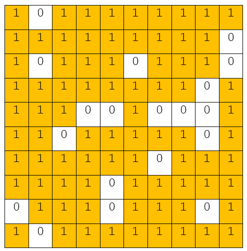
At each iteration, the algorithm generates the antenna based on design variables, computes S-parameters, and evaluates the objective function to obtain the population with the best cost value. The iterations continue until an optimized design is obtained.

Create Unit Pixel Patches

Create 100 small rectangular patches of size 1.758-by-1.385 mm each.

inputs.rows = 10;
inputs.cols = 10;
inputs.patchLength = 17.58e-3;
inputs.patchWidth = 13.85e-3;
inputs.unitPatches = cell(inputs.rows, inputs.cols);
inputs.unitPatchLength = inputs.patchLength/inputs.cols;
inputs.unitPatchWidth = (inputs.patchWidth/inputs.rows);
inputs.unitPatchCenters = [];
inputs.overlapWidth = 0.2e-3;% lo: Small margin to keep connection intact
inputs.commCenterX = -inputs.patchLength/2;
inputs.commCenterY = -inputs.groundPlaneWidth/2+inputs.f1Width+inputs.f2Width;

for i = 1:inputs.rows
    for j = 1:inputs.cols
        % Define pixels
        inputs.unitPatches{i, j} = antenna.Rectangle(Length=inputs.unitPatchLength+inputs.overlapWidth/2, ...
            Width=inputs.unitPatchWidth+inputs.overlapWidth/2, ...
            Center=[(i-1)*inputs.unitPatchLength+inputs.unitPatchLength/2+inputs.commCenterX (j-1)*inputs.unitPatchWidth+inputs.unitPatchWidth/2+inputs.commCenterY]);
        inputs.unitPatchCenters = [inputs.unitPatchCenters; inputs.unitPatches{i, j}.Center];        
    end
end

Define Objective Function

Create the radiating patch by adding the small patch when its design variable value is 1. When two diagonally adjacent patches have a value of $[\begin{array}{c} 0 & 1 \\ 1 & 0 \end{array}]$ or $[\begin{array}{c} 1 & 0 \\ 0 & 1 \end{array}]$ , their connection at the corner is too infinitesimal to ensure the electrical connectivity. To avoid this problem, specify that such patches overlap by 0.2 mm.

Next, define the objective function. The objective function is given by:

$cost = {\begin{cases} | S_{11} (f_{i}) | \exp (- 20 | \frac{f_{res} - f_{d}}{f_{d}} |), & f_{d} - ϵ < f_{i} < f_{d} + ϵ \\ | \frac{1}{N} \sum_{i = 1}^{N} S_{11} (i) | & otherwise \end{cases}$

$f_{i}$ is the Sampling frequency, $N$ is the total number of sampling points, $f_{d}$ is the desired frequency, $f_{res}$ is the individual resonance frequency, $S_{11}$ is the S-parameters of the antenna at resonance frequency, and $ϵ$ is 0.1.

function val = objectiveFunction(inputs, designVector)
%objectiveFunction evaluates the main goal of optimization and passes the
%output back to the optimizer for each iteration.

% Reshape the input from optimizer into a 10 X 10 matrix
designVector = reshape(designVector, 10, 10);
designVector(5:6,1) = 1;

patchNew = copy(inputs.feedArea);

% Add pixels in the patch top layer when value is 1
    for i = 1:inputs.rows
        for j = 1:inputs.cols
            if designVector(i, j) == 1 
                patchNew = patchNew + inputs.unitPatches{i, j};
            end
        end
    end

    % Add overlap when [1 0;0 1] or [0 1; 1 0]
    for i = 1:inputs.rows-1
        for j = 1:inputs.cols-1
            dV4 = designVector(i:i+1,j:j+1);
            if all(all(dV4 == [1 0;0 1])) || all(all(dV4 ==[0 1;1 0]))
                overlap = antenna.Rectangle(Length=2*inputs.unitPatchLength,Width=inputs.overlapWidth,...
                    Center=[i*inputs.unitPatchLength+inputs.commCenterX, j*inputs.unitPatchWidth+inputs.commCenterY]);
                patchNew = patchNew + overlap;
            end
        end
    end


    % Create pcbStack
    ant = pcbStack(Layers={patchNew, inputs.Subs inputs.ground}, BoardThickness=inputs.height, ...
        BoardShape=inputs.ground, FeedLocations=[inputs.feedLocation(1:2), 1, 3]);

    % Objective function

    N = 10; % Total sampling points
    fd = 2.16e9; % Desired frequency
    epsilon = 0.1e9; % Upper - Lower margin
    f =  linspace(fd-epsilon, fd+epsilon, N); % Sampling frequency

    s = sparameters(ant, f);
    S11 = rfparam(s,1,1); % S11(dB) parameter at resonance frequency
    cost = 0;

    for i = 1:N
        fres = f(i); % The individual resonance frequency        
        cost = cost + abs(S11(i))*exp(-20*abs((fres-fd)/fd));
    end
    val = cost;

end

GA Optimization

Use the ga (Global Optimization Toolbox) function to apply genetic algorithm optimization. Specify options for the function by using optimoptions. At each iteration:

- Plot best value of the objective function.

- Set the UseParallel flag to true (requires a Parallel Computing Toolbox™ license).

- Pass the objective function to the ga function with 100 design variables, the bounds [0,1], and the options structure.

The objective function that ga uses is given in the objectiveFunction method.

figure
% Optimization Options
options = optimoptions('ga',UseParallel=true,PlotFcn='gaplotbestf');
[x, fval, exitflag, output, population, scores] = ...
    ga(@(inputMat)objectiveFunction(inputs, inputMat), ...
    inputs.rows*inputs.cols, ... % Number of design variables
    [], [], [], [], ... % No linear constraints input
    zeros(1, inputs.rows*inputs.cols), ... % lower bound
    1.*ones(1, inputs.rows*inputs.cols), ... % upper bound
    [], ... % No nonlinear constraints
    1:inputs.rows*inputs.cols, ... % Integer constraint
    options); % options

Starting parallel pool (parpool) using the 'Processes' profile ...
Connected to parallel pool with 8 workers.
ga stopped because the average change in the penalty function value is less than options.FunctionTolerance and 
the constraint violation is less than options.ConstraintTolerance.

Optimized Antenna

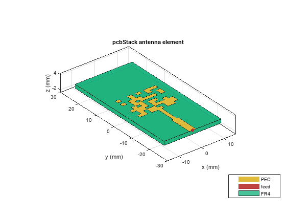
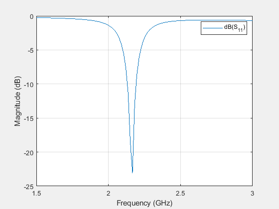
Create the optimized radiating patch by adding the small patches when ga output variable x is 1 with the overlap. Use pcbStack to create the optimized antenna, compute S-parameters, and observe the resonant frequency (which is around 2.16 GHz). Each run of this example leads to a new antenna structure, however the results remain same. Approximate execution time to obtain the optimized antenna is about 14 hours on a Windows® CPU @ 3.19 GHz system with 48 GB of RAM and 8 parallel workers.

designVector = x;
designVector = reshape(designVector, 10, 10);
designVector(5:6,1) = 1;
patchNew = copy(inputs.feedArea);

% Add pixels in the patch top layer when value = 1
for i = 1:inputs.rows
    for j = 1:inputs.cols
        if designVector(i, j) == 1 
            patchNew = patchNew + inputs.unitPatches{i, j};
        end
    end
end

% Add overlap when [1 0;0 1] or [0 1; 1 0]
for i = 1:inputs.rows-1
    for j = 1:inputs.cols-1
        dV4 = designVector(i:i+1,j:j+1);
        if all(all(dV4 == [1 0;0 1])) || all(all(dV4 ==[0 1;1 0]))
            overlap = antenna.Rectangle(Length=2*inputs.unitPatchLength,Width=inputs.overlapWidth,...
                Center=[i*inputs.unitPatchLength+inputs.commCenterX, j*inputs.unitPatchWidth+inputs.commCenterY]);
            patchNew = patchNew + overlap;
        end
    end
end

% Create the pcbStack
optimizedAnt = pcbStack(Layers={patchNew, inputs.Subs inputs.ground},BoardThickness=inputs.height, ...
    BoardShape=inputs.ground, FeedLocations=[inputs.feedLocation(1:2), 1, 3]);

figure
show(optimizedAnt);

Figure contains an axes object. The axes object with title pcbStack antenna element, xlabel x (mm), ylabel y (mm) contains 6 objects of type patch, surface. These objects represent PEC, feed, FR4.

sparams = sparameters(optimizedAnt,linspace(2e9,2.5e9,100));
figure
rfplot(sparams);

$Figure contains an axes object. The axes object with xlabel Frequency (GHz), ylabel Magnitude (dB) contains an object of type line. This object represents dB(S_{11}).$

Create Conventional Microstrip Patch Antenna at 2.16 GHz

Create a microstrip antenna of size 42-by-3.7 mm on an FR4 substrate with the thickness of 1.6 mm and a stepped microstrip feed to resonate around 2.16 GHz.

% Ground plane parameters
inputs.groundPlaneLength = 60e-3; 
inputs.groundPlaneWidth = 70e-3;

% Feed location
inputs.feedLocation = [0, -inputs.groundPlaneWidth/2, inputs.height];

% Create the feed strip
f1 = antenna.Rectangle(Length=inputs.f1Length, ...
    Width=inputs.f1Width, ...
    Center=[0, -inputs.groundPlaneWidth/2+inputs.f1Width/2]);
f2 = antenna.Rectangle(Length=inputs.f2Length, ...
    Width=inputs.f2Width, ...
    Center=[0, -inputs.groundPlaneWidth/2+inputs.f1Width+inputs.f2Width/2]);
inputs.feedArea = f1 + f2;

% Create the ground plane
inputs.ground = antenna.Rectangle(Length=inputs.groundPlaneLength, ...
    Width=inputs.groundPlaneWidth,Center=[0 0]);

patchRect2GHz = antenna.Rectangle(Length=42e-3,Width=33.7e-3,Center=[0, -inputs.groundPlaneWidth/2+inputs.f1Width+inputs.f2Width+33.7e-3/2]);

finalPatch2GHz  = inputs.feedArea + patchRect2GHz; 

antAt2GHz = pcbStack(Layers={finalPatch2GHz, inputs.Subs inputs.ground}, ...
    BoardThickness=inputs.height, ...
    BoardShape=inputs.ground, ...
    FeedLocations=[inputs.feedLocation(1:2), 1, 3]);

figure
show(antAt2GHz);

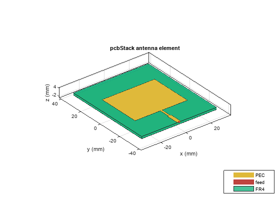
Figure contains an axes object. The axes object with title pcbStack antenna element, xlabel x (mm), ylabel y (mm) contains 6 objects of type patch, surface. These objects represent PEC, feed, FR4.

figure
rfplot(sparameters(antAt2GHz,linspace(1.5e9,3e9,100)));

$Figure Genetic Algorithm contains an axes object. The axes object with xlabel Frequency (GHz), ylabel Magnitude (dB) contains an object of type line. This object represents dB(S_{11}).$

Compare Optimized Antenna with Conventional Antenna

Compare the sizes of optimized and conventional microstrip antennas by plotting the patches side-by-side. Compared to the conventional microstrip antenna, the optimized microstrip antenna shows a patch size reduction of 82.79%.

fig = figure;
show(antAt2GHz.Layers{1});
hold on
translate(optimizedAnt.Layers{1},[35e-3 0 0]);
% Add annotation
annotation(fig,textbox=[0.17 0.16 0.16 0.094],String={'Conventional Antenna'},EdgeColor=[1 1 1]);
annotation(fig,textbox=[0.60 0.2 0.25 0.064],String={'Optimized Antenna'},EdgeColor=[1 1 1]);

Figure contains an axes object. The axes object with xlabel x (m), ylabel y (m) contains 4 objects of type patch. These objects represent PEC, mypolygon.

References

[1] Herscovici, N., M.F. Osorio, and C. Peixeiro. “Miniaturization of Rectangular Microstrip Patches Using Genetic Algorithms.” IEEE Antennas and Wireless Propagation Letters 1 (2002): 94–97. https://doi.org/10.1109/LAWP.2002.805128.

[2] Lamsalli, Mohammed, Abdelouahab El Hamichi, Mohamed Boussouis, Naima Amar Touhami, and Tajeddin Elhamadi. “Genetic Algorithm Optimization for Microstrip Patch Antenna Miniaturization.” Progress In Electromagnetics Research Letters 60 (2016): 113–20. https://doi.org/10.2528/PIERL16041907.