Modeling Mutual Coupling in Large Arrays Using Infinite Array Analysis

Define Individual Element

For this example, the center of the X-band is chosen as the design frequency.

freq = 10e9;
vp = physconst('lightspeed');
lambda = vp/freq;
ucdx = 0.5*lambda;
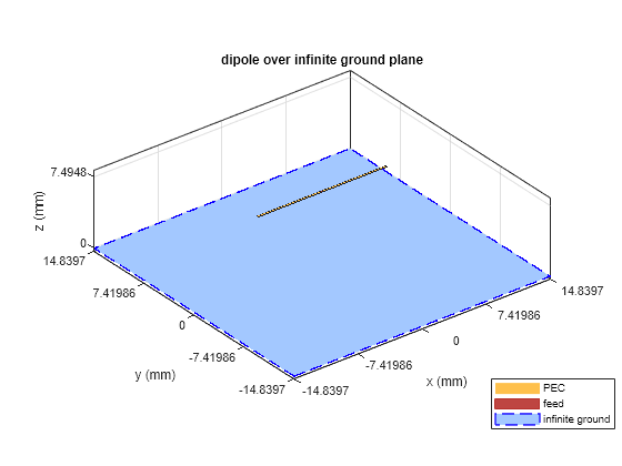
ucdy = 0.5*lambda;

Create a thin dipole of length slightly less than $$\lambda (lambda)/2$$ and assign it as the exciter to a infinitely large reflector.

d = dipole;
d.Length = 0.495*lambda;
d.Width = lambda/160;
d.Tilt = 90;
d.TiltAxis = [0 1 0];

r = reflector;
r.Exciter = d;
r.Spacing = lambda/4;
r.GroundPlaneLength = inf;
r.GroundPlaneWidth = inf;
figure;
show(r);

Calculate the isolated element pattern and the impedance of the above antenna. These results are used to calculate the Scan Element Pattern(SEP), also known as Array Element Pattern(AEP) or Embedded Element Pattern(EEP).

%Define az and el vectors
az = 0:2:360;
el = 90:-2:-90;

% Calculate power pattern
giso = pattern(r,freq,az,el,'Type','power');  % el x az

% Calculated impedance
Ziso = impedance(r,freq);

Calculate Infinite Array Scan Element Pattern

Unit cell

The term unit cell in the infinite array analysis refers to a single element in an infinite array. A dipole backed by a reflector and a microstrip patch antenna are representative examples of a unit cell in infinite arrays. This example uses a dipole backed by a reflector and analyzes the impedance behavior at 10 GHz as a function of the scan angle. The unit cell has a cross-section of $$\lambda /2$$-by-$$\lambda /2$$.

r.GroundPlaneLength = ucdx;
r.GroundPlaneWidth = ucdy;
infArray = infiniteArray;
infArray.Element = r;
infArray.ScanAzimuth = 30;
infArray.ScanElevation = 45;
figure;
show(infArray);

Scan impedance

The scan impedance at a single frequency and single scan angle is shown.

scanZ = impedance(infArray,freq)

scanZ = 1.0862e+02 + 3.0435e+01i

For this example, the scan impedance for the full volume of scan is calculated using 50 terms in the double summation for the periodic Greens function to improve convergence behavior. For more information, refer to the following example: Infinite Array Analysis.

Scan Element Pattern /Array Element Pattern /Embedded Element Pattern

The scan element pattern (SEP) is calculated from the infinite array scan impedance, the isolated element pattern and the isolated element impedance. The expression used is shown here[1],[2]:

load InfArrayScanZData
scanZ = scanZ.';
Rg = 185;             
Xg = 0;
Zg = Rg + 1i*Xg;
gs = nan(numel(el),numel(az));
for i = 1:numel(el) 
    for j = 1:numel(az)
    gs(i,j) = 4*Rg*real(Ziso).*giso(i,j)./(abs(scanZ(i,j) + Zg)).^2;
    end
end

Build Custom Antenna Element

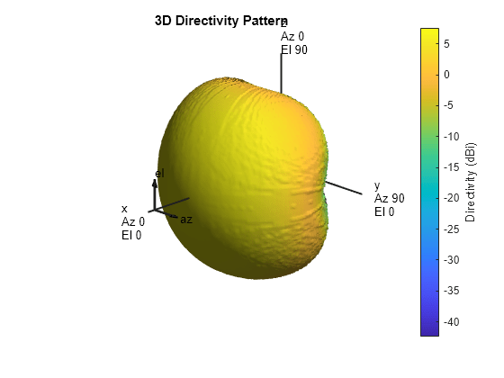
The scan element pattern obtained from full-wave analysis is now used in a system level analysis provided by the Phased Array System Toolbox™. For that, build a custom antenna element as a first step.

fieldpattern = sqrt(gs);
bandwidth = 500e6;
customAntInf = buildCustomAntenna(fieldpattern,freq,bandwidth,az,el);
figure;
pattern(customAntInf,freq);

Build 21-by-21 URA

Create a uniform rectangular array (URA) with the custom antenna element, which contains the scan element pattern. The assumption implicit in this step is that every element of this array has the same element pattern.

N = 441;
Nrow = sqrt(N);
Ncol = sqrt(N);
drow = ucdx;
dcol = ucdy;
myURA1 = phased.URA;
myURA1.Element = customAntInf;
myURA1.Size = [Nrow Ncol];
myURA1.ElementSpacing = [drow dcol];

Plot Slices in E and H planes

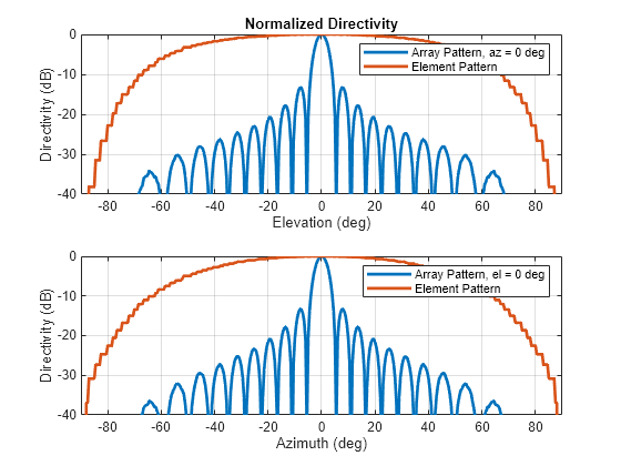
Calculate the pattern in the elevation plane (specified by azimuth = 0 deg and also called the E-plane) and azimuth plane (specified by elevation = 0 deg and called the H-plane) for the array built using infinite array analysis.

azang_plot = -90:0.5:90;
elang_plot = -90:0.5:90;
% E-plane
Darray1_E = pattern(myURA1,freq,0,elang_plot);
Darray1_Enormlz = Darray1_E - max(Darray1_E);
% H-plane
Darray1_H = pattern(myURA1,freq,azang_plot,0);
Darray1_Hnormlz = Darray1_H - max(Darray1_H);
% Scan element pattern in both planes
DSEP1_E = pattern(customAntInf,freq,0,elang_plot);
DSEP1_Enormlz = DSEP1_E - max(DSEP1_E);
DSEP1_H = pattern(customAntInf,freq,azang_plot,0);
DSEP1_Hnormlz = DSEP1_H - max(DSEP1_H);

figure
subplot(211)
plot(elang_plot,Darray1_Enormlz,elang_plot,DSEP1_Enormlz,'LineWidth',2)
grid on
axis([min(azang_plot) max(azang_plot) -40 0]);
legend('Array Pattern, az = 0 deg','Element Pattern')
xlabel('Elevation (deg)')
ylabel('Directivity (dB)')
title('Normalized Directivity')
subplot(212)
plot(azang_plot,Darray1_Hnormlz,azang_plot,DSEP1_Hnormlz,'LineWidth',2)
grid on
axis([min(azang_plot) max(azang_plot) -40 0]);
legend('Array Pattern, el = 0 deg','Element Pattern')
xlabel('Azimuth (deg)')
ylabel('Directivity (dB)')

Comparison with Full Wave Finite Array Analysis

To understand the effect of the finite size of the array, we execute a full wave analysis of a 21 X 21 dipole array backed by an infinite reflector. The full wave array pattern slices in the E and H planes as well as the center element embedded element pattern is also calculated. This data is loaded from a MAT file. This analysis took approximately 630 seconds on a 2.4 GHz machine with 32 GB memory.

Load full wave data and build custom antenna

Load the finite array analysis data, and use the embedded element pattern to build a custom antenna element. Note that the pattern from the full-wave analysis needs to be rotated by 90 degrees so that it lines up with the URA model built on the YZ plane.

load dipolerefarray
elemfieldpatternfinite = sqrt(FiniteArrayPatData.ElemPat);
arraypatternfinite = FiniteArrayPatData.ArrayPat;
bandwidth = 500e6;
customAntFinite = buildCustomAntenna(elemfieldpatternfinite,freq,bandwidth,az,el);
figure
pattern(customAntFinite,freq)

Create Uniform Rectangular Array with embedded element pattern

As done before, create a uniform rectangular array with the custom antenna element.

myURA2 = phased.URA;
myURA2.Element = customAntFinite;
myURA2.Size = [Nrow Ncol];
myURA2.ElementSpacing = [drow dcol];

E and H plane slice - array With embedded element pattern

Calculate the pattern slices in two orthogonal planes - E and H for the array with the embedded element pattern and the embedded element pattern itself. In addition, since the full wave data for the array pattern is also available use this to compare results.

Darray2_E = pattern(myURA2,freq,0,elang_plot);
Darray2_Enormlz = Darray2_E - max(Darray2_E);
% H-plane
Darray2_H = pattern(myURA2,freq,azang_plot,0);
Darray2_Hnormlz = Darray2_H - max(Darray2_H);

E and H plane slice - embedded element pattern from finite array

DSEP2_E = pattern(customAntFinite,freq,0,elang_plot);
DSEP2_Enormlz = DSEP2_E - max(DSEP2_E);
DSEP2_H = pattern(customAntFinite,freq,azang_plot,0);
DSEP2_Hnormlz = DSEP2_H - max(DSEP2_H);

E and H plane slice - full wave analysis of finite array

azang_plot1 = -90:2:90;
elang_plot1 = -90:2:90;

Darray3_E = FiniteArrayPatData.EPlane;
Darray3_Enormlz = Darray3_E - max(Darray3_E);

Darray3_H = FiniteArrayPatData.HPlane;
Darray3_Hnormlz = Darray3_H - max(Darray3_H);

Comparison of array patterns

The array patterns in the two orthogonal planes are plotted here.

figure
subplot(211)
plot(elang_plot,Darray1_Enormlz,elang_plot,Darray2_Enormlz,elang_plot1,Darray3_Enormlz,'LineWidth',2)
grid on
axis([min(elang_plot) max(elang_plot) -40 0]);
legend('Infinite','Finite','Finite Full wave','location','best')
xlabel('Elevation (deg)')
ylabel('Directivity (dB)')
title('E-plane (az=0 deg) Normalized Array Directivity')
subplot(212)
plot(azang_plot,Darray1_Hnormlz,azang_plot,Darray2_Hnormlz,azang_plot1,Darray3_Hnormlz,'LineWidth',2)
grid on
axis([min(azang_plot) max(azang_plot) -40 0]);
legend('Infinite','Finite','Finite Full wave','location','best')
xlabel('Azimuth (deg)')
ylabel('Directivity (dB)')
title('H-Plane (el = 0 deg) Normalized Array Directivity')

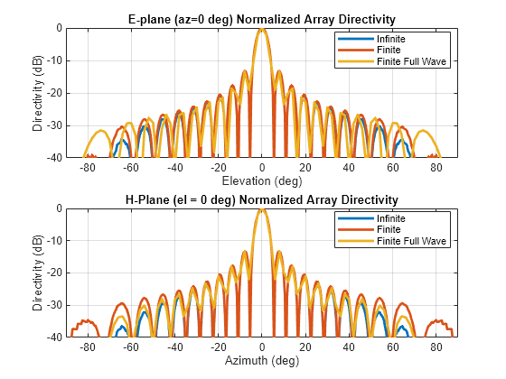
The pattern plots in the two planes reveals that all three analysis approaches suggest similar behavior out to +/-40 degree from boresight. Beyond this range, it appears that using the scan element pattern for all elements in a URA (i.e. pattern multiplication principle) underestimates the sidelobe level compared to the full wave analysis of a finite array. The one possible reason for this could be the edge effect from the finite size array.

Comparison of element patterns

The element patterns from the infinite array analysis and the finite array analysis are compared here.

figure
subplot(211)
plot(elang_plot,DSEP1_Enormlz,elang_plot,DSEP2_Enormlz,'LineWidth',2)
grid on
axis([min(azang_plot) max(azang_plot) -40 0]);
legend('Infinite','Finite','location','best')
xlabel('Elevation (deg)')
ylabel('Directivity (dB)')
title('E-plane (az=0 deg) Normalized Element Directivity')
subplot(212)
plot(azang_plot,DSEP1_Hnormlz,azang_plot,DSEP2_Hnormlz,'LineWidth',2)
grid on
axis([min(azang_plot) max(azang_plot) -40 0]);
legend('Infinite','Finite','location','best')
xlabel('Azimuth (deg)')
ylabel('Directivity (dB)')
title('H-Plane (el = 0 deg) Normalized Element Directivity')

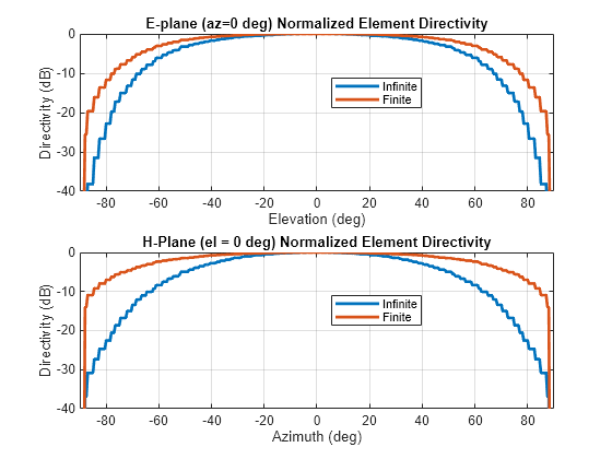
The pattern plots suggests that the behavior out to +/-40 degree from boresight is approximately the same. Outside of this range there is greater drop off in the H-plane pattern from the infinite array analysis as compared to the finite array.

Scan Behavior with Infinite Array Scan Element Pattern

Scan the array based on the infinite array scan element pattern in the elevation plane defined by azimuth = 0 deg and plot the normalized directivity. Also, overlay the normalized scan element pattern.

scanURA(myURA1,freq,azang_plot,elang_plot,DSEP1_Enormlz,DSEP1_Hnormlz);

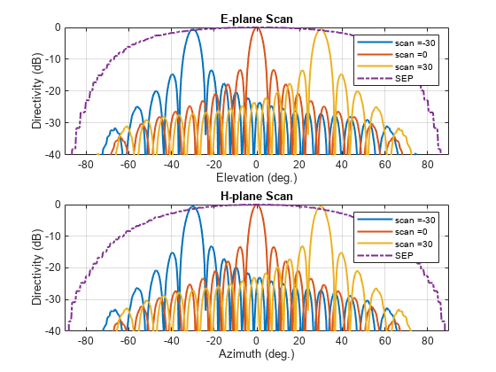
Note the overall shape of the normalized array pattern approximately follows the normalized scan element pattern. This is also predicted by the pattern multiplication principle.

Conclusion

Infinite array analysis is one of the tools deployed to analyze and design large finite arrays. The analysis assumes that all elements are identical, have uniform excitation amplitude and that edge effects can be ignored. The isolated element pattern is replaced with the scan element pattern which includes the effect of mutual coupling.

Reference

[1] J. Allen, "Gain and impedance variation in scanned dipole arrays," IRE Transactions on Antennas and Propagation, vol.10, no.5, pp.566-572, September 1962.

[2] R. C. Hansen, Phased Array Antennas, Chapter 7 and 8, John Wiley & Sons Inc.,2nd Edition, 1998.