Main Content

acousticRoughness

Perceived roughness of acoustic signal

Since R2021a

Description

roughness = acousticRoughness(audioIn,fs) returns roughness strength in aspers based on Zwicker [1] and ISO 532-1 time-varying loudness [2].

example

roughness = acousticRoughness(audioIn,fs,calibrationFactor) specifies a nondefault microphone calibration factor used to compute loudness.

example

roughness = acousticRoughness(specificLoudnessIn) computes roughness using high-resolution time-varying specific loudness.

example

roughness = acousticRoughness(___,Name,Value) specifies options using one or more Name, Value pair arguments. For example, roughness = acousticRoughness(audioIn,fs,'SoundField','diffuse') returns roughness assuming a diffuse sound field.

example

[roughness,specificRoughness] = acousticRoughness(___) also returns specific roughness strength.

[roughness,specificRoughness,fMod] = acousticRoughness(___) also returns the dominant modulation frequency detected by the algorithm.

acousticRoughness(___) with no output arguments plots roughness strength and specific roughness strength and displays the modulation frequency textually. If audioIn is stereo, the 3-D plot shows the sum of both channels.

example

Examples

collapse all

Measure acoustic roughness based on [1] and ISO 532-1 [2]. Assume a free-field reference pressure of 20 micropascals and a recording level calibration such that a 1 kHz tone registers as 100 dB on a SPL meter.

Read in a stereo audio file and convert to mono.

[audioInStereo,fs] = audioread('Engine-16-44p1-stereo-20sec.wav');
audioIn = (audioInStereo(:,1) + audioInStereo(:,2)) / 2;

Compute acoustic roughness on the mono audio signal and display the average value.

roughness = acousticRoughness(audioIn,fs);
meanRoughness = mean(roughness);
displayOutput = ['Average computed value of acoustic roughness is ',num2str(meanRoughness),' aspers.'];
disp(displayOutput)
Average computed value of acoustic roughness is 0.17901 aspers.

References

[1] Zwicker, Eberhard, and Hugo Fastl. Psychoacoustics: Facts and Models. Vol. 22. Springer Science & Business Media, 2013.

[2] ISO 532-1:2017(E). "Acoustics – Methods for calculating loudness – Part 1: Zwicker method." International Organization for Standardization.

Set up an experiment as indicated by the diagram.

Create an audioDeviceReader object to read from the microphone and an audioDeviceWriter object to write to your speaker.

fs = 48e3;
deviceReader = audioDeviceReader(fs,"SamplesPerFrame",2048);
deviceWriter = audioDeviceWriter(fs);

Create an audioOscillator object to generate a 1 kHz sinusoid.

osc = audioOscillator("sine",1e3,"SampleRate",fs,"SamplesPerFrame",2048);

Create a dsp.AsyncBuffer object to buffer data acquired from the microphone.

dur = 5;
buff = dsp.AsyncBuffer(dur*fs);

For 5 seconds, play the sinusoid through your speaker and record using your microphone. While the audio streams, note the loudness as reported by your SPL meter. Once complete, read the contents of the buffer object.

numFrames = dur*(fs/osc.SamplesPerFrame);
for ii = 1:numFrames
    audioOut = osc();
    deviceWriter(audioOut);
    
    audioIn = deviceReader();
    write(buff,audioIn);
end

SPLreading = 69.7;

micRecording = read(buff);

To compute the calibration factor for the microphone, use the calibrateMicrophone function.

calibrationFactor = calibrateMicrophone(micRecording(fs+1:end),deviceReader.SampleRate,SPLreading);

You can now use the calibration factor you determined to measure the roughness of any sound that is acquired through the same microphone recording chain.

Perform the experiment again by adding 100% amplitude modulation at 40 Hz. To create the modulation signal, use the audioOscillator object and specify the amplitude as 0.5 and the DC offset as 0.5 to oscillate between 0 and 1.

mod = audioOscillator("sine",40,"SampleRate",fs, ...
    "Amplitude",0.5,"DCOffset",0.5,"SamplesPerFrame",2048);

dur = 5;
buff = dsp.AsyncBuffer(dur*fs);
numFrames = dur*(fs/osc.SamplesPerFrame);
for ii = 1:numFrames
    audioOut = osc().*mod();
    deviceWriter(audioOut);
    
    audioIn = deviceReader();
    write(buff,audioIn);
end

micRecording = read(buff);

Call the acousticRoughness function with the microphone recording, sample rate, and calibration factor. The roughness reported from acousticRoughness uses the true acoustic loudness measurement as specified by ISO 532-1. Display the average roughness strength over the 5 seconds and plot roughness and specific roughness.

roughness = acousticRoughness(micRecording,deviceReader.SampleRate,calibrationFactor);
fprintf('Average roughness = %d (asper)',mean(roughness(2001:end,:)))
Average roughness = 4.992723e-01 (asper)
acousticRoughness(micRecording,deviceReader.SampleRate,calibrationFactor)

Read in an audio file.

[audioIn,fs] = audioread("Engine-16-44p1-stereo-20sec.wav");

Call the acousticLoudness function using high time resolution to calculate the specific loudness.

[~,specificLoudnessHD] = acousticLoudness(audioIn,fs,'TimeVarying',true,'TimeResolution','high');

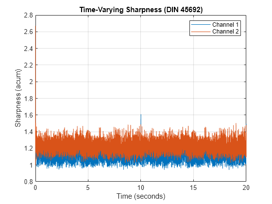
Call the acousticSharpness function using standard resolution specific loudness without any output arguments to plot the acoustic sharpness.

specificLoudness = specificLoudnessHD(1:4:end,:,:);
acousticSharpness(specificLoudness,'TimeVarying',true)

Figure contains an axes object. The axes object with title Time-Varying Sharpness (DIN 45692), xlabel Time (seconds), ylabel Sharpness (acum) contains 2 objects of type line. These objects represent Channel 1, Channel 2.

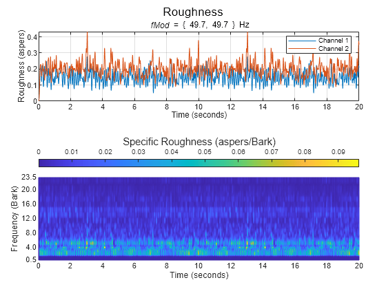
Call acousticRoughness without any outputs to plot the acoustic roughness.

acousticRoughness(specificLoudnessHD)

Figure contains 2 axes objects and another object of type subplottext. Axes object 1 with title fMod blank = blank { blank 49 . 7 , blank 49 . 7 blank } Hz, xlabel Time (seconds), ylabel Roughness (aspers) contains 2 objects of type line. These objects represent Channel 1, Channel 2. Axes object 2 with xlabel Time (seconds), ylabel Frequency (Bark) contains an object of type surface.

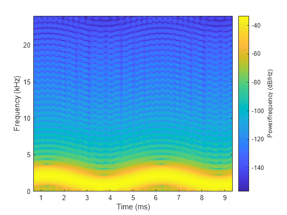
Generate a pure tone with a 1500 Hz center frequency and approximately 700 Hz frequency deviation at a modulation frequency of 200 Hz.

fs = 48e3;

fMod = 200;
dur = 5;

numSamples = dur*fs;
t = (0:numSamples-1)/fs;

tone = sin(2*pi*t*fMod)';

fc = 1500;
excursionRatio = 0.47;

excursion = 2*pi*(fc*excursionRatio/fs);
audioIn = modulate(tone,fc,fs,'fm',excursion);

Listen to the audio and plot a spectrogram of the first 10 ms.

sound(audioIn,fs)
spectrogram(audioIn(1:0.01*fs),hann(64,'periodic'),63,1024,fs,'yaxis')

Figure contains an axes object. The axes object with xlabel Time (ms), ylabel Frequency (kHz) contains an object of type image.

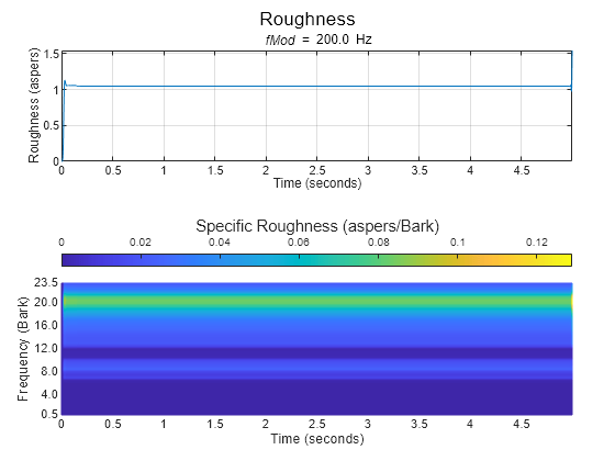
Call the acousticRoughness function with no output arguments to plot the acoustic roughness strength.

acousticRoughness(audioIn,fs);

Figure contains 2 axes objects and another object of type subplottext. Axes object 1 with title fMod blank = blank 200 . 0 Hz, xlabel Time (seconds), ylabel Roughness (aspers) contains an object of type line. Axes object 2 with xlabel Time (seconds), ylabel Frequency (Bark) contains an object of type surface.

The acousticRoughness function enables you to specify a known roughness frequency. If you do not specify a known roughness frequency, the function auto detects the roughness.

Create a dsp.AudioFileReader object to read in an audio signal frame-by-frame. Create an audioOscillator object to create a modulation wave. Apply the modulation wave to the audio file.

fileReader = dsp.AudioFileReader('Engine-16-44p1-stereo-20sec.wav');

fMod = 72.41;
amplitude = 0.5;

osc = audioOscillator('sine',fMod, ...
    "DCOffset",0.5, ...
    "Amplitude",amplitude, ...
    "SampleRate",fileReader.SampleRate, ...
    "SamplesPerFrame",fileReader.SamplesPerFrame);

testSignal = [];
while ~isDone(fileReader)
    x = fileReader();
    testSignal = [testSignal;osc().*fileReader()];
end

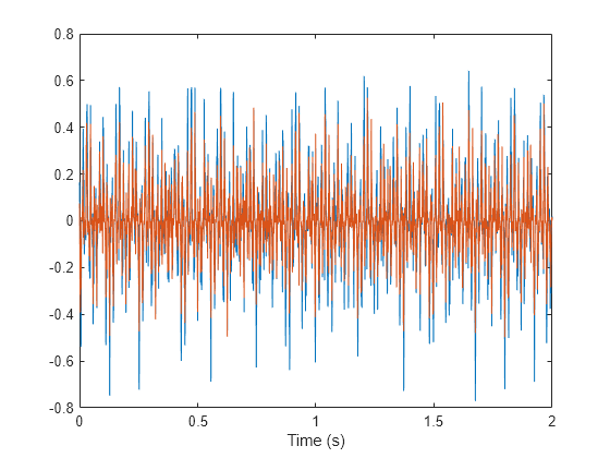
Listen to 2 seconds of the test signal and plot its waveform.

samplesToView = 1:2*fileReader.SampleRate;
sound(testSignal(samplesToView,:),fileReader.SampleRate);

plot(samplesToView/fileReader.SampleRate,testSignal(samplesToView,:))
xlabel('Time (s)')

Figure contains an axes object. The axes object with xlabel Time (s) contains 2 objects of type line.

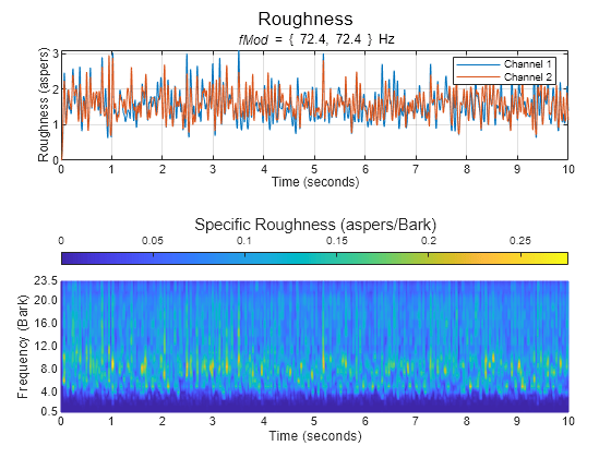
Plot the acoustic roughness. The detected frequency of the modulation is displayed textually.

acousticRoughness(testSignal,fileReader.SampleRate);

Figure contains 2 axes objects and another object of type subplottext. Axes object 1 with title fMod blank = blank { blank 72 . 4 , blank 72 . 4 blank } Hz, xlabel Time (seconds), ylabel Roughness (aspers) contains 2 objects of type line. These objects represent Channel 1, Channel 2. Axes object 2 with xlabel Time (seconds), ylabel Frequency (Bark) contains an object of type surface.

Specify the known modulation frequency and then plot the acoustic roughness again.

acousticRoughness(testSignal,fileReader.SampleRate,'ModulationFrequency',fMod)

Figure contains 2 axes objects and another object of type subplottext. Axes object 1 with title fMod blank = blank { blank 72 . 4 , blank 72 . 4 blank } Hz, xlabel Time (seconds), ylabel Roughness (aspers) contains 2 objects of type line. These objects represent Channel 1, Channel 2. Axes object 2 with xlabel Time (seconds), ylabel Frequency (Bark) contains an object of type surface.

Input Arguments

collapse all

Audio input, specified as a column vector (mono) or matrix with two columns (stereo).

Tip

To measure roughness strength given any modulation frequency, the recommended minimum signal duration is 0.5 seconds.

Data Types: single | double

Sample rate in Hz, specified as a positive scalar. The recommended sample rate for new recordings is 48 kHz.

Note

The minimum acceptable sample rate is 8 kHz.

Data Types: single | double

Microphone calibration factor, specified as a positive scalar. The default calibration factor corresponds to a full-scale 1 kHz sine wave with a sound pressure level of 100 dB (SPL). To compute the calibration factor specific to your system, use the calibrateMicrophone function.

Data Types: single | double

Specific loudness in sones/Bark, specified as a T-by-240-by-C array, where:

  • T is 1 per 0.5 ms of the time-varying signal (high resolution loudness).

  • 240 is the number of Bark bins in the domain for specific loudness. The Bark bins are 0.1:0.1:24.

  • C is the number of channels.

You can use the acousticLoudness function to calculate time varying specific loudness using this syntax.

[~,specificLoudness] = acousticLoudness(audioIn,fs,'TimeVarying',true,'TimeResolution','high');

Data Types: single | double

Name-Value Arguments

Specify optional pairs of arguments as Name1=Value1,...,NameN=ValueN, where Name is the argument name and Value is the corresponding value. Name-value arguments must appear after other arguments, but the order of the pairs does not matter.

Before R2021a, use commas to separate each name and value, and enclose Name in quotes.

Example: acousticRoughness(audioIn,fs,'ModulationFrequency',100)

Known modulation frequency in Hz, specified as the comma-separated pair consisting of 'ModulationFrequency' and a scalar or two-element vector with values in the range [1,1000].

Set ModulationFrequency to:

  • 'auto-detect' when you want the function to detect the modulation frequency automatically. When you select this option the function limits the search range to between 10 and 400 Hz.

  • a scalar if the input is mono.

  • a scalar or two-element vector if the input is stereo.

Data Types: single | double | char | string

Sound field of audio recording, specified as the comma-separated pair of 'SoundField' and 'free' or 'diffuse'.

Data Types: char | string

Reference pressure for dB calculation in pascals, specified as the comma-separated pair of 'PressureReference' and a positive scalar. The default value, 20 micropascals, is the common value of air.

Data Types: single | double

Output Arguments

collapse all

Roughness strength in asper, returned as a K-by-1 column vector or K-by-2 matrix of independent channels. K corresponds to the time dimension.

Note

Roughness is reported for each channel independently at every 0.5 ms interval.

Data Types: single | double

Specific roughness strength in asper/Bark, returned as a K-by-47 matrix or a K-by-47-by-2 array. The first dimension of specificRoughness, K, corresponds to the time dimension and matches the first dimension of roughness. The second dimension of specificRoughness, 47, corresponds to bands on the Bark scale, with centers in the range of [0.5, 23.5], in increments of 0.5. The third dimension of specificRoughness corresponds to the number of channels and matches the second dimension of roughness.

Data Types: single | double

Dominant modulation frequency in Hz, returned as a scalar for mono input or a 1-by-2 vector for stereo input.

Data Types: single | double

Algorithms

Acoustic roughness strength is a perceptual measurement of modulations in amplitude or frequency that are too high to discern separately. The acoustic loudness algorithm is described in [2] and implemented in the acousticLoudness function. The acoustic roughness calculation is described in [1]. The algorithm for acoustic roughness defines the roughness of 1 asper as a 1 kHz tone at 60 dB with a 100% amplitude modulation at 70 Hz [3]. The algorithm is outlined as follows:

roughness=calz=024fmodΔLdz

Where fmod is the detected or known modulation frequency, cal is a constant ensuring unity roughness of the reference signal, and ΔL is the perceived modulation depth. If the modulation frequency is not specified when calling acousticRoughness, it is auto-detected by peak-picking a frequency-domain representation of the acoustic loudness. The perceived modulation depth ΔL is calculated by passing rectified specific loudness bands through ½ octave filters centered around fmod, followed by a lowpass filter to determine the envelope.

References

[1] Zwicker, Eberhard, and Hugo Fastl. Psychoacoustics: Facts and Models. Vol. 22. Springer Science & Business Media, 2013.

[2] ISO 532-1:2017(E). "Acoustics – Methods for calculating loudness – Part 1: Zwicker method." International Organization for Standardization.

[3] Kalafata, Stamatina. "Sound Levels, Noise Source Identification and Perceptual Analysis in an Intensive Care Unit." Master's thesis, University of Gothenburg, 2014.

Extended Capabilities

Version History

Introduced in R2021a