acousticLoudness
Perceived loudness of acoustic signal
Syntax
Description
loudness = acousticLoudness(audioIn,fs,calibrationFactor)
loudness = acousticLoudness(___,Name,Value)Name,Value pair arguments.
Example: loudness = acousticLoudness(audioIn,fs,'Method','ISO
532-2') returns loudness according to ISO 532-2
(Moore-Glasberg).
[
also returns the specific loudness.loudness,specificLoudness] = acousticLoudness(___)
[
also returns percentile loudness.loudness,specificLoudness,perc] = acousticLoudness(___,'TimeVarying',true)
[
specifies nondefault percentiles to return.loudness,specificLoudness,perc] = acousticLoudness(___,'TimeVarying',true,'Percentiles',p)
acousticLoudness(___) with no output arguments plots
specific loudness and displays loudness textually. If TimeVarying is
true, both loudness and specific loudness are plotted, with the
latter in 3-D.
Examples
Measure the ISO 532-1 stationary free-field loudness. Assume the recording level is calibrated such that a 1 kHz tone registers as 100 dB on a SPL meter.
[audioIn,fs] = audioread('WashingMachine-16-44p1-stereo-10secs.wav');

loudness = acousticLoudness(audioIn,fs)
loudness = 1×2
28.2688 27.7643
Create two stationary signals with equivalent power: a pink noise signal and a white noise signal.
fs = 48e3;
dur = 5;
pnoise = 2*pinknoise(dur*fs);
wnoise = rand(dur*fs,1) - 0.5;
wnoise = wnoise*sqrt(var(pnoise)/var(wnoise));
Call acousticLoudness using the default ISO 532-1 (Zwicker) method and no output arguments to plot the loudness of the pink noise. Call acousticLoudness again, this time with output arguments, to get the specific loudness.
figure
acousticLoudness(pnoise,fs)
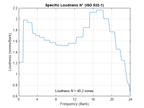
ans =
40.1941
[~,pSpecificLoudness] = acousticLoudness(pnoise,fs);
Plot the loudness for the white noise signal and then get the specific loudness values.
figure
acousticLoudness(wnoise,fs)
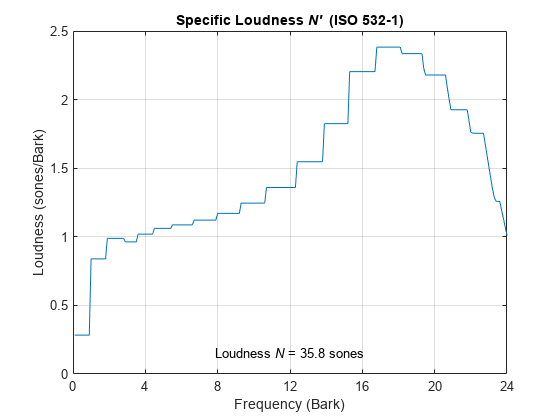
ans =
35.8379
[~,wSpecificLoudness] = acousticLoudness(wnoise,fs);
Call the acousticSharpness function to compare the sharpness of the pink noise and white noise.
pSharpness = acousticSharpness(pSpecificLoudness);
wSharpness = acousticSharpness(wSpecificLoudness);
fprintf('Sharpness of pink noise = %0.2f acum\n',pSharpness)
Sharpness of pink noise = 2.00 acum
fprintf('Sharpness of white noise = %0.2f acum\n',wSharpness)Sharpness of white noise = 2.62 acum
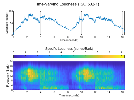
Read in an audio file.
[audioIn,fs] = audioread('JetAirplane-16-11p025-mono-16secs.wav');Plot the time-varying acoustic loudness in accordance with ISO 532-1 and get the percentiles. Listen to the audio signal.
acousticLoudness(audioIn,fs,'SoundField','diffuse','TimeVarying',true)
ans = 8174×1

         0
    0.0715
    1.5794
    3.5609
    5.1448
    6.2449
    7.1623
    7.7970
    8.3737
    8.9203
    9.1421
    9.3955
    9.6771
    9.8421
   10.1413
      ⋮
sound(audioIn,fs)
Call acousticLoudness again with the same inputs and get the percentiles. Print the Nmax and N5 percentiles. The Nmax percentile is the maximum loudness reported. The N5 percentile is the loudness below which is 95% of the reported loudness.
[~,~,perc] = acousticLoudness(audioIn,fs,'SoundField','diffuse','TimeVarying',true);
fprintf('Max loudness = %0.2f sones\n',perc(1))
Max loudness = 89.48 sones
fprintf('N5 loudness = %0.2f sones\n',perc(2))N5 loudness = 81.77 sones
Read in an audio file.
[audioIn,fs] = audioread('Turbine-16-44p1-mono-22secs.wav');Call acousticLoudness with no output arguments to plot the specific loudness. Assume a calibration factor of 0.15 and a reference pressure of 21 micropascals. To determine the calibration factor specific to your audio system, use the calibrateMicrophone function.
calibrationFactor = 0.15;
refPressure = 21e-6;
acousticLoudness(audioIn,fs,calibrationFactor,'PressureReference',refPressure)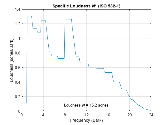
ans =
15.1672
acousticLoudness enables you to specify an intermediate representation, sound pressure levels, instead of a time-domain input. This enables you to reuse intermediate SPL calculations. Another advantage is that if your physical SPL meter does not report loudness in accordance to ISO 532-1 or ISO 531-2, you can use the reported 1/3-octave SPLs to calculate standard-compliant loudness.
To calculate sound pressure levels from an audio signal, first create an splMeter object. Call the splMeter object with the audio input.
spl = splMeter("SampleRate",fs,"Bandwidth","1/3 octave", ...
    "CalibrationFactor",calibrationFactor,"PressureReference",refPressure, ...
    "FrequencyWeighting","Z-weighting","OctaveFilterOrder",6);

splMeasurement = spl(audioIn);
Compute the mean SPL level, skipping the first 0.2 seconds. Only keep the bands from 25 Hz to 12.5 kHz (the first 28 bands).
SPLIn = mean(splMeasurement(ceil(0.2*fs):end,1:28));
Using the SPL input, call acousticLoudness with no output arguments to plot the specific loudness.
acousticLoudness(SPLIn)

ans =
15.2003
Set up an experiment as indicated by the diagram.
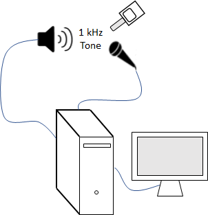
Create an audioDeviceReader object to read from the microphone and an audioDeviceWriter object to write to your speaker.
fs = 48e3;
deviceReader = audioDeviceReader(fs);
deviceWriter = audioDeviceWriter(fs);
Create an audioOscillator object to generate a 1 kHz sinusoid.
osc = audioOscillator("sine",1e3,"SampleRate",fs);
Create a dsp.AsyncBuffer object to buffer data acquired from the microphone.
dur = 5;
buff = dsp.AsyncBuffer(dur*fs);
For five seconds, play the sinusoid through your speaker and record using your microphone. While the audio streams, note the loudness as reported by your SPL meter. Once complete, read the contents of the buffer object.
numFrames = dur*(fs/osc.SamplesPerFrame);
for ii = 1:numFrames
    audioOut = osc();
    deviceWriter(audioOut);

    audioIn = deviceReader();
    write(buff,audioIn);
end

SPLreading = 60.4;

micRecording = read(buff);
To compute the calibration factor for the microphone, use the calibrateMicrophone function.
calibrationFactor = calibrateMicrophone(micRecording,deviceReader.SampleRate,SPLreading);
Call acousticLoudness with the microphone recording, sample rate, and calibration factor. The loudness reported from acousticLoudness is the true acoustic loudness measurement as specified by 532-1.
loudness = acousticLoudness(micRecording,deviceReader.SampleRate,calibrationFactor)
loudness =
14.7902
You can now use the calibration factor you determined to measure the loudness of any sound that is acquired through the same microphone recording chain.
Read in an audio signal.
[audioIn,fs] = audioread('TrainWhistle-16-44p1-mono-9secs.wav');ISO 532-1
Determine the time-varying specific loudness according to the default method (ISO 532-1).
[~,specificLoudness] = acousticLoudness(audioIn,fs,'TimeVarying',true);ISO 532-1 reports specific loudness over Bark, where the Bark bins are 0.1:0.1:24. Convert the Bark bins to Hz and then plot the specific loudness over Hz across time.
barkBins = 0.1:0.1:24;
hzBins = bark2hz(barkBins);

t = 0:2e-3:2e-3*(size(specificLoudness,1)-1);
surf(t,hzBins,sum(specificLoudness,3).','EdgeColor','interp')
set(gca,'YScale','log')
view([0 90])
axis tight
xlabel('Time (s)')
ylabel('Frequency (Hz)')
colorbar
title('Specific Loudness (sones/Bark)')

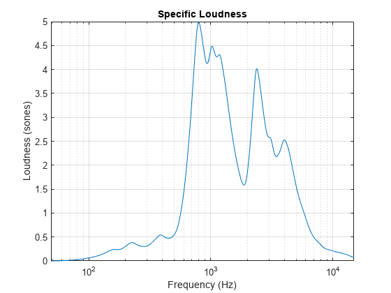
ISO 532-2
Determine the stationary specific loudness according to the Moore-Glasberg method (ISO 532-2).
[~,specificLoudness] = acousticLoudness(audioIn,fs,'Method','ISO 532-2');
ISO 532-2 reports specific loudness over the ERB scale, where the ERB bins are 1.8:0.1:38.9. The unit of the ERB scale is sometimes referred to as Cam. Convert the ERB bins to Hz and then plot the specific loudness.
erbBins = 1.8:0.1:38.9;
hzBins = erb2hz(erbBins);

semilogx(hzBins,specificLoudness)
xlabel('Frequency (Hz)')
ylabel('Loudness (sones)')
title('Specific Loudness')
grid on
Read in an audio file.
[x,fs] = audioread('WashingMachine-16-44p1-stereo-10secs.wav');ISO 532-2 enables you to specify a custom earphone response when calculating loudness. Create a 30-by-2 matrix where the first column is the frequency and the second column is the earphone's deviation from a flat response.
tdh = [   0,    80,   100,  200,  500,  574,  660,  758,  871, 1000, 1149,  1320,  1516,  1741,  2000, ...
       2297,  2639,  3031, 3482, 4000, 4500, 5000, 5743, 6598, 7579, 8706, 10000, 12000, 16000, 20000; ...
        -50, -15.3, -13.8, -8.1, -0.5,  0.4,  0.8,  0.9,  0.5,  0.1, -0.8,  -1.5,  -2.3,  -3.2,  -3.9, ...
       -4.2,  -4.3,  -4.3, -3.9, -3.2, -2.3, -1.1, -0.3,   -2, -5.4,   -9, -12.1, -15.2,   -30,   -50 ].';
Calculate the loudness using ISO 532-2. Specify SoundField as earphones and the earphone response as the matrix you just created.
acousticLoudness(x,fs,'Method','ISO 532-2','SoundField','earphones','EarphoneResponse',tdh)
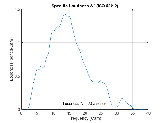
ans =
20.3199
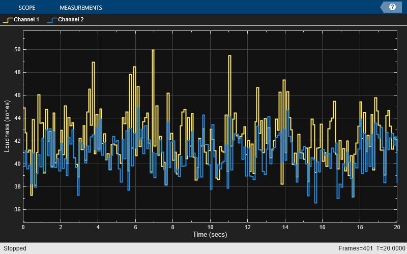
Create a dsp.AudioFileReader object to read in an audio signal frame-by-frame. Specify a frame duration of 50 ms. This will be the frame duration over which you calculate stationary loudness.
fileReader = dsp.AudioFileReader('Engine-16-44p1-stereo-20sec.wav');

frameDur = 0.05;
fileReader.SamplesPerFrame = round(fileReader.SampleRate*frameDur);
Create an audioDeviceWriter object to write audio to your default output device.
deviceWriter = audioDeviceWriter('SampleRate',fileReader.SampleRate);Create a timescope object to display stationary loudness over time.
scope = timescope( ...
    'SampleRate',1/frameDur, ...
    'YLabel','Loudness (sones)', ...
    'ShowGrid',true, ...
    'PlotType','Stairs', ...
    'TimeSpanSource','property', ...
    'TimeSpan',20, ...
    'AxesScaling','Auto', ...
    'ShowLegend',true);
In a loop:
Read a frame from the audio file.
Calculate the stationary loudness of that frame.
Play the sound through your output device.
Write the loudness to the scope.
while ~isDone(fileReader)
    audioIn = fileReader();
    loudness = acousticLoudness(audioIn,fileReader.SampleRate);
    deviceWriter(audioIn);
    scope(loudness)
end
release(fileReader)
release(deviceWriter)
release(scope)
Input Arguments
Name-Value Arguments
Output Arguments
Algorithms
Loudness and loudness level are perceptual attributes of sound. Due to differences among people, measurements of loudness and loudness level should be considered statistical estimators. The ISO 532 series specifies procedures for estimating loudness and loudness level as perceived by persons with ontologically normal hearing under specific listening conditions.
ISO 532-1 and ISO 532-2 specify two different methods for calculating loudness, but leave it to the user to select the appropriate method for a given situation.
ISO 532-1:2017(E) describes methods for calculating acoustic loudness of stationary and time-varying signals.
This method is based on DIN 45631:1991. The algorithm differs from ISO 532:1975, method B, by specifying corrections for low frequencies.
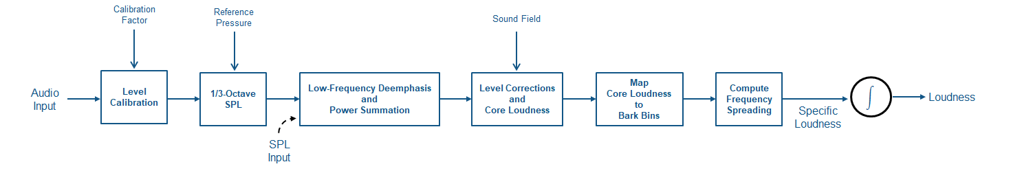
The diagram and the steps provide a high-level overview of the sequence of the method. For details, see [1].
The time-domain signal level is adjusted according to the
CalibrationFactor. The following steps of the algorithm assume a true known signal level.The signal is transformed to a 1/3 octave SPL representation using fractional octave band filtering. The filter bank consists of 28 filters between 25 Hz to 12.5 kHz. The output from this stage is in dB and normalized by the reference pressure.
Low frequency 1/3 octave bands are de-emphasized according to a fixed weighting table. Some of the low-frequency bands are combined to form a total of 20 critical bands.
The levels of the critical bands are corrected for filter bandwidth and the critical band level at the threshold of quiet, and then transformed to core loudness.
Core loudness is mapped to Bark bins.
Frequency spreading is computed using a table of level- and frequency-dependent slopes.
Loudness is calculated as the integral of specific loudness, taking into account the frequency-spreading slopes.
This method is based on DIN 45631/A1:2010, and is designed to properly simulate the duration-dependent behavior of loudness perception for short impulses. The method for time-varying sounds is a generalization of the Zwicker approach to stationary signals. If the generalized version is applied to stationary sounds, it gives the same loudness values as the non-generalized form for stationary signals.
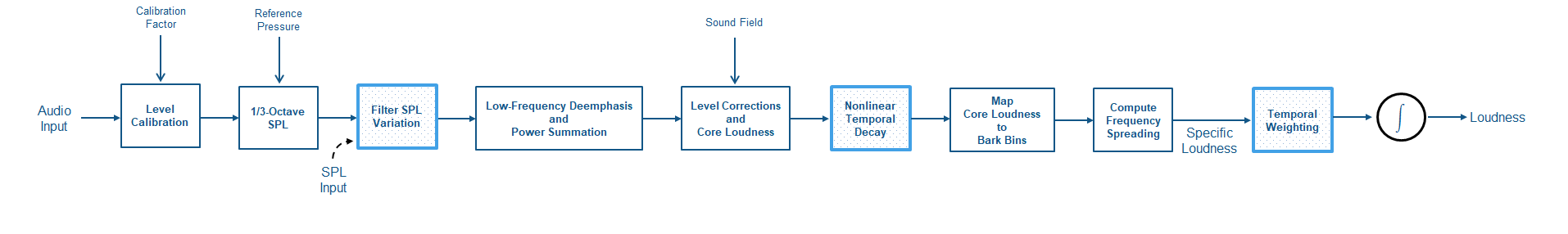
The diagram and the steps provide a high-level overview of the sequence of the method. For details, see [1].
The time-domain signal level is adjusted according to the
CalibrationFactor. The following steps of the algorithm assume a true known signal level.The signal is transformed to a 1/3 octave SPL representation using fractional octave band filtering. The filter bank consists of 28 filters between 25 Hz to 12.5 kHz. The output from this stage is in dB and normalized by the reference pressure.
The SPL bands are smoothed along time according to band-dependent filters.
Low frequency 1/3 octave bands are de-emphasized according to a fixed weighting table. Some of the low-frequency bands are combined to form a total of 20 critical bands.
The levels of the critical bands are corrected for filter bandwidth and the critical band level at the threshold of quiet, and then transformed to core loudness.
Nonlinear temporal decay is simulated using a diode-capacitor-resistor network. This models the steep perceptual drop after short signals when compared to long signals.
Core loudness is mapped to Bark bins.
Frequency spreading is computed using a table of level- and frequency-dependent slopes.
Temporal weighting is applied to simulate the duration-dependence of loudness perception.
Loudness is calculated as the integral of specific loudness, taking into account the frequency-spreading slopes.
ISO 532-2:2017(E) describes a binaural model for calculating acoustic loudness of stationary signals. The method in ISO 523-2 differs from those in ISO 532:1975: it improves the calculated loudness in the low frequency range and the binaural model allows for different sounds for each ear. ISO 532-2 provides a good match to the equal loudness level contours defined in ISO 226:2003, and the threshold of hearing defined in ISO 389-7:2005.
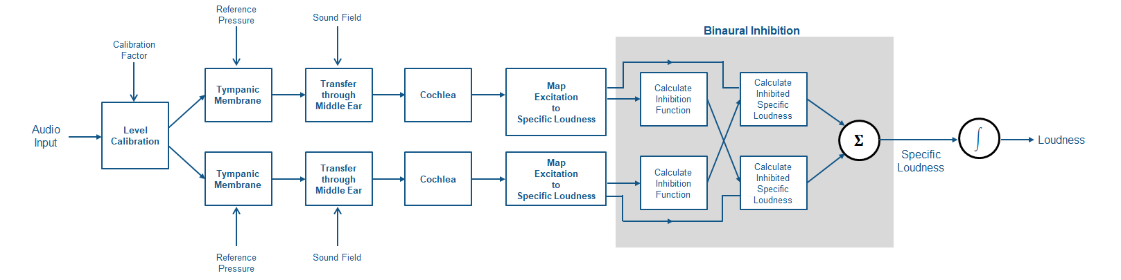
The diagram and the steps provide a high-level overview of the sequence of the method. For details, see [2].
The time-domain signal level is adjusted according to the
CalibrationFactor. The following steps of the algorithm assume a true known signal level.The signal is transformed to a spectral representation. The spectral representation is transformed according to fixed filters representing the transfer of sound through the tympanic membrane (eardrum). The spectrum is scaled according to the reference pressure.
The signal is transformed using a model of the inner ear. Again, the transfer function is given by a fixed filter specified in the standard. The filter choice depends on the specified sound field.
The signal is transformed from the sound spectrum to an excitation pattern at the basilar membrane. The transformation is accomplished using a series of rounded-exponential filters spread on the ERB scale.
The excitation pattern is converted to specific loudness.
The specific loudness is passed through a model of binary inhibition, where a signal at one ear inhibits the loudness evoked by a signal at the other ear. The output from this stage is the specific loudness in sones/ERB.
The specific loudness is integrated over the ERB scale to give the loudness in sones.
References
[1] ISO 532-1:2017(E). "Acoustics – Methods for calculating loudness – Part 1: Zwicker method." International Organization for Standardization.
[2] ISO 532-2:2017(E). "Acoustics – Methods for calculating loudness – Part 2: Moore-Glasberg method. International Organization for Standardization.
Extended Capabilities
Version History
Introduced in R2020a