Accelerate Audio Deep Learning Using GPU-Based Feature Extraction

This example uses:

In this example, you leverage a GPU for feature extraction and augmentation to decrease the time required to train a deep learning model. The model you train is a convolutional neural network (CNN) for acoustic fault recognition.

Audio Toolbox™ includes gpuArray (Parallel Computing Toolbox) support for most feature extractors, including popular ones such as melSpectrogram and mfcc. For an overview of GPU support, see Code Generation and GPU Support.

Load Training Data

Download and unzip the air compressor data set [1]. This data set consists of recordings from air compressors in a healthy state or one of seven faulty states.

downloadFolder = matlab.internal.examples.downloadSupportFile("audio","AirCompressorDataset/AirCompressorDataset.zip");
dataFolder = tempdir;
unzip(downloadFolder,dataFolder)
dataset = fullfile(dataFolder,"AirCompressorDataset");

Create an audioDatastore object to manage the data and split it into training and validation sets.

ads = audioDatastore(dataset,IncludeSubfolders=true,LabelSource="foldernames");
rng default
[adsTrain,adsValidation] = splitEachLabel(ads,0.8);

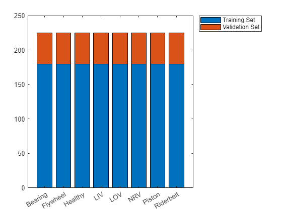
Visualize the number of files in the training and validation sets.

uniqueLabels = unique(adsTrain.Labels);
tblTrain = countEachLabel(adsTrain);
tblValidation = countEachLabel(adsValidation);
H = bar(uniqueLabels,[tblTrain.Count, tblValidation.Count],"stacked");
legend(H,["Training Set","Validation Set"],Location="NorthEastOutside")

Select random examples from the training set for plotting. Each recording has 50,000 samples sampled at 16 kHz.

t = (0:5e4-1)/16e3;
tiledlayout(4,2,TileSpacing="compact",Padding="compact")
for n = 1:numel(uniqueLabels)
    idx = find(adsTrain.Labels==uniqueLabels(n));
    [x,fs] = audioread(adsTrain.Files{idx(randperm(numel(idx),1))});

    nexttile
    plotHandle = plot(t,x);
    if n == 7 || n == 8
        xlabel("Seconds");
    else
        set(gca,xtick=[])
    end
    title(string(uniqueLabels(n)));
end

Preprocess Data on CPU and GPU

In this example, you perform feature extraction and data augmentation while training the network. In this section, you define the feature extraction and augmentation pipeline and compare the speed of the pipeline executed on a CPU against the speed of the pipeline executed on a GPU. The output of this pipeline is the input to the CNN you train.

Create an audioFeatureExtractor object to extract log-mel spectrums using 200 ms mel windows with a 5 ms hop. The output from extract is a numHops-by-128-by-1 array.

afe = audioFeatureExtractor(SampleRate=fs, ...
    FFTLength=4096, ...
    Window=hann(round(fs*0.2),"periodic"), ...
    OverlapLength=round(fs*0.195), ...
    melSpectrum=true);
setExtractorParameters(afe,"melSpectrum",NumBands=128,ApplyLog=true);

featureVector = extract(afe,x);
[numHops,numFeatures,numChannels] = size(featureVector)

numHops = 586

numFeatures = 128

numChannels = 1

Deep learning methods are data-hungry, and the training dataset in this example is relatively small. Use the mixup [2] augmentation technique to effectively enlarge the training set. In mixup, you merge the features extracted from two audio signals as a weighted sum. The two signals have different labels, and the label assigned to the merged feature matrix is probabilistically assigned based on the mixing coefficient. The mixup augmentation is implemented in the supporting object, Mixup.

Create the pipeline to perform the following steps:

Extract the log-mel spectrogram.
Apply mixup to the feature matrices. The Mixup supporting object outputs a cell array containing the features and the label.

Create two versions of the pipeline for comparison: one that executes the pipeline on your CPU, and one that converts the raw audio signal to a gpuArray so that the pipeline is executed on your GPU.

offset = eps;

adsTrainCPU = transform(adsTrain,@(x)extract(afe,x));
mixerCPU = Mixup(adsTrainCPU);
adsTrainCPU = transform(adsTrainCPU,@(x,info)mix(mixerCPU,x,info),IncludeInfo=true);

adsTrainGPU = transform(adsTrain,@gpuArray);
adsTrainGPU = transform(adsTrainGPU,@(x)extract(afe,x));
mixerGPU = Mixup(adsTrainGPU);
adsTrainGPU = transform(adsTrainGPU,@(x,info)mix(mixerGPU,x,info),IncludeInfo=true);

For the validation set, apply the feature extraction pipeline but not the augmentation. Because you are not applying mixup, create a combined datastore to output a cell array containing the features and the label. Again, create one validation pipeline that executes on your GPU and one validation pipeline that executes on your CPU.

adsValidationGPU = transform(adsValidation,@gpuArray);
adsValidationGPU = transform(adsValidationGPU,@(x){extract(afe,x)});
adsValidationGPU = combine(adsValidationGPU,arrayDatastore(adsValidation.Labels));

adsValidationCPU = transform(adsValidation,@(x){extract(afe,x)});
adsValidationCPU = combine(adsValidationCPU,arrayDatastore(adsValidation.Labels));

Compare the time it takes for the CPU and a single GPU to extract features and perform data augmentation.

tic
for ii = 1:numel(adsTrain.Files)
    x = read(adsTrainCPU);
end
cpuPipeline = toc;
reset(adsTrainCPU)

tic
for ii = 1:numel(adsTrain.Files)
    x = read(adsTrainGPU);
end
wait(gpuDevice) % Ensure all calculations are completed
gpuPipeline = toc;
reset(adsTrainGPU)

disp(["Read, extract, and augment train set (CPU): "+cpuPipeline+" seconds"; ...
    "Read, extract, and augment train set (GPU): "+gpuPipeline+" seconds"; ...
    "Speedup (CPU time)/(GPU time): "+cpuPipeline/gpuPipeline]);

    "Read, extract, and augment train set (CPU): 119.2114 seconds"
    "Read, extract, and augment train set (GPU): 25.5192 seconds"
    "Speedup (CPU time)/(GPU time): 4.6714"

Reading from the datastore contributes a significant amount of the overall time to the pipeline. A comparison of just extraction and augmentation shows an even greater speedup. Compare just feature extraction on the GPU versus on the CPU.

x = read(ads);

extract(afe,x); % Incur initialization cost outside timing loop
tic
for ii = 1:numel(adsTrain.Files)
    features = extract(afe,x);
end
cpuFeatureExtraction = toc;

x = gpuArray(x); % Incur initialization cost outside timing loop
extract(afe,x);
tic
for ii = 1:numel(adsTrain.Files)
    features = extract(afe,x);
end
wait(gpuDevice) % Ensure all calculations are completed
gpuFeatureExtraction = toc;

disp(["Extract features from train set (CPU): "+cpuFeatureExtraction+" seconds"; ...
    "Extract features from train set (GPU): "+gpuFeatureExtraction+" seconds"; ...
    "Speedup (CPU time)/(GPU time): "+cpuFeatureExtraction/gpuFeatureExtraction]);

    "Extract features from train set (CPU): 52.015 seconds"
    "Extract features from train set (GPU): 1.184 seconds"
    "Speedup (CPU time)/(GPU time): 43.9302"

Define Network

Define a convolutional neural network that takes the augmented mel spectrogram as input. This network applies a single convolutional layer consisting of 48 filters with 3-by-3 kernels, followed by a batch normalization layer and a ReLU activation layer. The time dimension is then collapsed using a max pooling layer. Finally, the output of the pooling layer is reduced using a fully connected layer followed by softmax layer. See List of Deep Learning Layers (Deep Learning Toolbox) for more information.

numClasses = numel(categories(adsTrain.Labels));
imageSize = [numHops,afe.FeatureVectorLength];

layers = [
    imageInputLayer(imageSize,Normalization="none")

    convolution2dLayer(3,48,Padding="same")
    batchNormalizationLayer
    reluLayer

    maxPooling2dLayer([numHops,1])

    fullyConnectedLayer(numClasses)
    softmaxLayer
    ];

To define the training options, use trainingOptions (Deep Learning Toolbox). Set the ExecutionEnvironment to gpu to leverage your GPU while training the network. The computer used in this example uses a Titan V GPU device.

miniBatchSize = 128;
options = trainingOptions("adam", ...
    Shuffle="every-epoch", ...
    MaxEpochs=20, ...
    LearnRateSchedule="piecewise", ...
    LearnRateDropPeriod=15, ...
    LearnRateDropFactor=0.2, ...
    MiniBatchSize=miniBatchSize, ...
    Plots="training-progress", ...
    Verbose=false, ...
    ValidationData=adsValidationCPU, ...
    ValidationFrequency=2*ceil(numel(adsTrain.Files)/miniBatchSize), ...
    ExecutionEnvironment="gpu", ...
    Metrics="accuracy");

Train Network

Train Network Using CPU-Based Preprocessing

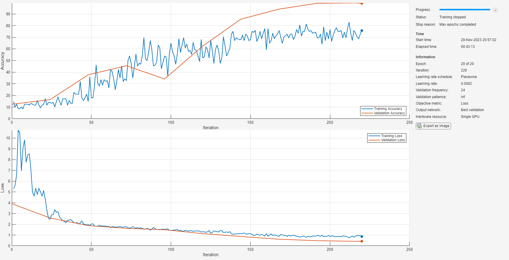
Call trainnet to train the network using your CPU for the feature extraction pipeline. The execution environment for the network training is your GPU.

tic
net = trainnet(adsTrainCPU,layers,"crossentropy",options);

cpuTrainTime = toc;

Train Network Using GPU-Based Preprocessing

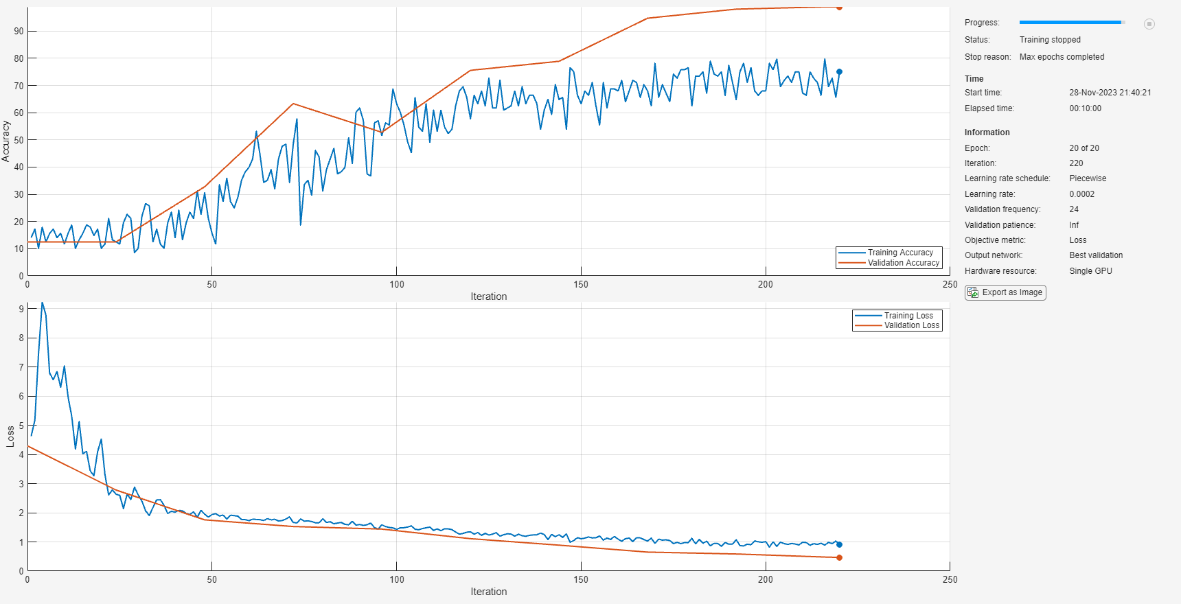
Replace the validation data in the training options with the GPU-based pipeline. Train the network using your GPU for the feature extraction pipeline. The execution environment for the network training is your GPU.

options.ValidationData = adsValidationGPU;
tic
net = trainnet(adsTrainGPU,layers,"crossentropy",options);

gpuTrainTime = toc;

Compare CPU- and GPU-based Preprocessing

Print the timing results for training using a CPU for feature extraction and augmentation, and training using a GPU for feature extraction and augmentation.

disp(["Training time (CPU): "+cpuTrainTime+" seconds";
    "Training time (GPU): "+gpuTrainTime+" seconds";
    "Speedup (CPU time)/(GPU time): "+cpuTrainTime/gpuTrainTime])

    "Training time (CPU): 2611.0347 seconds"
    "Training time (GPU): 604.3813 seconds"
    "Speedup (CPU time)/(GPU time): 4.3202"

Compare CPU and GPU Inference Performance

Compare the time it takes to perform prediction on a single 3-second clip when feature extraction is performed on the GPU versus the CPU. In both cases, the network prediction happens on your GPU.

signalToClassify = read(ads);

gpuFeatureExtraction = gputimeit(@()predict(net,extract(afe,gpuArray(signalToClassify))));
cpuFeatureExtraction = gputimeit(@()predict(net,extract(afe,(signalToClassify))));

disp(["Prediction time for 3 s of data (feature extraction on CPU): "+cpuFeatureExtraction*1e3+" ms"; ...
    "Prediction time for 3 s of data (feature extraction on GPU): "+gpuFeatureExtraction*1e3+" ms"; ...
    "Speedup (CPU time)/(GPU time): "+cpuFeatureExtraction/gpuFeatureExtraction])

    "Prediction time for 3 s of data (feature extraction on CPU): 45.2426 ms"
    "Prediction time for 3 s of data (feature extraction on GPU): 7.0415 ms"
    "Speedup (CPU time)/(GPU time): 6.4251"

Compare the time it takes to perform prediction on a set of 3-second clips when feature extraction is performed on the GPU versus the CPU. In both cases, the network prediction happens on your GPU.

adsValidationGPU = transform(adsValidation,@(x)gpuArray(x));
adsValidationGPU = transform(adsValidationGPU,@(x){extract(afe,x)});
adsValidationCPU = transform(adsValidation,@(x){extract(afe,x)});

gpuFeatureExtraction = gputimeit(@()minibatchpredict(net,adsValidationGPU,ExecutionEnvironment="gpu"));
cpuFeatureExtraction = gputimeit(@()minibatchpredict(net,adsValidationCPU,ExecutionEnvironment="gpu"));

disp(["Prediction time for validation set (feature extraction on CPU): "+cpuFeatureExtraction+" seconds";
    "Prediction time for validation set (feature extraction on GPU): "+gpuFeatureExtraction+" seconds";
    "Speedup (CPU time)/(GPU time): "+cpuFeatureExtraction/gpuFeatureExtraction])

    "Prediction time for validation set (feature extraction on CPU): 15.8432 seconds"
    "Prediction time for validation set (feature extraction on GPU): 2.4479 seconds"
    "Speedup (CPU time)/(GPU time): 6.4722"

Conclusion

It is well known that you can decrease the time it takes to train a network by leveraging GPU devices. This enables you to more quickly iterate and develop your final system. In many training setups, you can achieve additional performance gains by leveraging GPU devices for feature extraction and data augmentation. This example shows a significant decrease in the overall time it takes to train a CNN when leveraging GPU devices for feature extraction and data augmentation. Additionally, leveraging GPU devices for feature extraction at inference time, for both single-observations and data sets, achieves significant performance gains.

Supporting Functions

Mixup

The supporting object, Mixup, is placed in your current folder when you open this example.

type Mixup

classdef Mixup < handle
    %MIXUP Mixup data augmentation
    %   mixer = Mixup(augDatastore) creates an object that can mix features
    %   at a randomly set ratio and then probabilistically set the output
    %   label as one of the two original signals.
    %
    %   Mixup Properties:
    %   MixProbability - Mix probability
    %   AugDatastore   - Augmentation datastore
    %
    %   Mixup Methods:
    %   mix            - Apply mixup
    %

    % Copyright 2021 The MathWorks, Inc.

    properties (SetAccess=public,GetAccess=public)
        %MixProbability Mix probability
        % Specify the probability that mixing is applied as a scalar in the
        % range [0,1]. If unspecified, MixProbability defaults to 1/3.
        MixProbability (1,1) {mustBeNumeric} = 1/3;
    end
    properties (SetAccess=immutable,GetAccess=public)
        %AUGDATASTORE Augmentation datastore
        % Specify a datastore from which to get the mixing signals. The
        % datastore must contain a label in the info returned from reading.
        % This property is immutable, meaning it cannot be changed after
        % construction.
        AugDatastore
    end

    methods
        function obj = Mixup(augDatastore)
            obj.AugDatastore = augDatastore;
        end

        function [dataOut,infoOut] = mix(obj,x,infoIn)
            %MIX Apply mixup
            % [dataOut,infoOut] = mix(mixer,x,infoIn) probabilistically mix
            % the input, x, and its associated label contained in infoIn
            % with a signal randomly drawn from the augmentation datastore.
            % The output, dataOut, is a cell array with two columns. The
            % first column contains the features and the second column
            % contains the label.

            if rand > obj.MixProbability % Only mix ~1/3 the dataset

                % Randomly set mixing coefficient. Draw from a normal
                % distribution with mean 0.5 and contained within [0,1].
                lambda = max(min((randn./10)+0.5,1),0);

                % Read one file from the augmentation datastore.
                subDS = subset(obj.AugDatastore,randi([1,numel(obj.AugDatastore.UnderlyingDatastores{1}.Files)]));
                [y,yInfo] = read(subDS);

                % Mix the features element-by-element according to lambda.
                dataOut = lambda*x + (1-lambda)*y;

                % Set the output label probabilistically based on the mixing coefficient.
                if lambda < rand
                    labelOut = yInfo.Label;
                    infoOut.Label = labelOut;
                else
                    labelOut = infoIn.Label;
                end
                infoOut.Label = labelOut;

                % Combine the output data and labels.
                dataOut = [{dataOut},{labelOut}];

            else % Do not apply mixing

                dataOut = [{x},{infoIn.Label}];
                infoOut = infoIn;

            end
        end

    end
end

References

[1] Verma, Nishchal K., et al. "Intelligent Condition Based Monitoring Using Acoustic Signals for Air Compressors." IEEE Transactions on Reliability, vol. 65, no. 1, Mar. 2016, pp. 291–309. DOI.org (Crossref), doi:10.1109/TR.2015.2459684.

[2] Huszar, Ferenc. "Mixup: Data-Dependent Data Augmentation." InFERENCe. November 03, 2017. Accessed January 15, 2019. https://www.inference.vc/mixup-data-dependent-data-augmentation/.