info
Characteristic information about fading channel object
Syntax
Description
Examples
Use the info object function to get information from a comm.RayleighChannel object.
Create a Rayleigh channel object with two paths and data to pass through the channel.
rayleighchan = comm.RayleighChannel( ...
    SampleRate=1000, ...
    PathDelays=[0 4e-3], ...
    AveragePathGains=[0 0])
rayleighchan =
  comm.RayleighChannel with properties:

             SampleRate: 1000
     PathGainSampleRate: 'signal'
             PathDelays: [0 0.0040]
       AveragePathGains: [0 0]
     NormalizePathGains: true
    MaximumDopplerShift: 1.0000e-03
        DopplerSpectrum: [1×1 struct]
       ChannelFiltering: true
    PathGainsOutputPort: false

  Show all properties
data = randi([0 1],600,1);
Check the Rayleigh channel object information.
info(rayleighchan)
ans = struct with fields:
    ChannelFilterCoefficients: [2×5 double]
           ChannelFilterDelay: 0
          NumSamplesProcessed: 0
           PathGainSampleRate: 1000
Pass data through the channel and check the object information again to see that the information structure accounts for the number of samples processed.
rayleighchan(data);
Sint = info(rayleighchan)
Sint = struct with fields:
    ChannelFilterCoefficients: [2×5 double]
           ChannelFilterDelay: 0
          NumSamplesProcessed: 600
           PathGainSampleRate: 1000
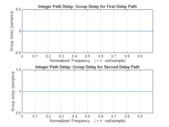
Breaking down the group delay per path, the specified PathDelays times SampleRate results in ([0 4e-3]*1000) = [0 4] sample path delays. Since the requested path delays are all integer-valued, the implemented channel filter adds no excess delay to the channel output, and the ChannelFilterDelay field reports 0 samples for the delay. As configured, the channel results in a constant group delay equal to (PathDelays*SampleRate + ChannelFilterDelay) = ([0 4e-3]*1000 + 0) = [0 4] samples per path. Use the grpdelay function to confirm the group delay for each path.
figure
subplot(2,1,1)
grpdelay(Sint.ChannelFilterCoefficients(1,:),1)
title('Integer Path Delay: Group Delay for First Delay Path')
subplot(2,1,2)
grpdelay(Sint.ChannelFilterCoefficients(2,:),1)
title('Integer Path Delay: Group Delay for Second Delay Path')

Release the object so you can update attributes. Change the second path delay to a noninteger value of 1.5e-3 seconds. Implementing a filter with a noninteger path delay introduces excess group delay. The info object function reports this excess delay in the ChannelFilterDelay field of the information structure. Recheck the object configuration and information.
release(rayleighchan)
rayleighchan.PathDelays = [0 1.5e-3]
rayleighchan =
  comm.RayleighChannel with properties:

             SampleRate: 1000
     PathGainSampleRate: 'signal'
             PathDelays: [0 0.0015]
       AveragePathGains: [0 0]
     NormalizePathGains: true
    MaximumDopplerShift: 1.0000e-03
        DopplerSpectrum: [1×1 struct]
       ChannelFiltering: true
    PathGainsOutputPort: false

  Show all properties
rayleighchan(data);
Snonint = info(rayleighchan)
Snonint = struct with fields:
    ChannelFilterCoefficients: [2×16 double]
           ChannelFilterDelay: 6
          NumSamplesProcessed: 600
           PathGainSampleRate: 1000
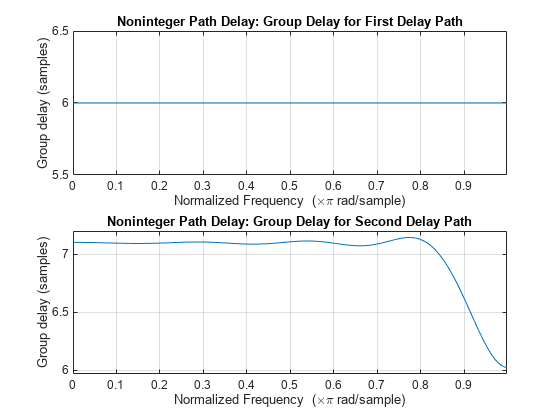
Breaking down the group delay per path, the specified PathDelays times SampleRate results in ([0 1.5e-3]*1000) = [0 1.5] sample path delays. Since the requested path delays contain at least one noninteger value, the channel filter implementation results in excess group delay at the channel output and the ChannelFilterDelay field now reports 6 samples for the delay. As configured, the channel results in a constant group delay equal to (PathDelays*SampleRate + ChannelFilterDelay) = ([0 1.5e-3]*1000 + 6) = [6 7.5] samples per path. Use the grpdelay function to confirm the group delay for each path.
figure
subplot(2,1,1)
grpdelay(Snonint.ChannelFilterCoefficients(1,:),1)
title('Noninteger Path Delay: Group Delay for First Delay Path')
subplot(2,1,2)
grpdelay(Snonint.ChannelFilterCoefficients(2,:),1)
title('Noninteger Path Delay: Group Delay for Second Delay Path')

Use the info object function to get information from a comm.RicianChannel object.
Create a Rician channel object with two paths and data to pass through the channel.
ricianchan = comm.RicianChannel( ...
    SampleRate=500, ...
    PathDelays=[0 2e-3], ...
    AveragePathGains=[0 0])
ricianchan =
  comm.RicianChannel with properties:

                SampleRate: 500
        PathGainSampleRate: 'signal'
                PathDelays: [0 0.0020]
          AveragePathGains: [0 0]
        NormalizePathGains: true
                   KFactor: 3
    DirectPathDopplerShift: 0
    DirectPathInitialPhase: 0
       MaximumDopplerShift: 1.0000e-03
           DopplerSpectrum: [1×1 struct]
          ChannelFiltering: true
       PathGainsOutputPort: false

  Show all properties
data = randi([0 1],600,1);
Check the Rician channel object information.
info(ricianchan)
ans = struct with fields:
    ChannelFilterCoefficients: [2×2 double]
           ChannelFilterDelay: 0
          NumSamplesProcessed: 0
           PathGainSampleRate: 500
Pass data through the channel and check the object information again to see that the information structure accounts for the number of samples processed.
ricianchan(data);
Sint = info(ricianchan)
Sint = struct with fields:
    ChannelFilterCoefficients: [2×2 double]
           ChannelFilterDelay: 0
          NumSamplesProcessed: 600
           PathGainSampleRate: 500
Breaking down the group delay per path, the specified PathDelays times SampleRate results in ([0 2e-3]*500) = [0 1] sample path delays. Since the requested path delays are all integer-valued, the implemented channel filter adds no excess delay to the channel output, and the ChannelFilterDelay field reports 0 samples for the delay. As configured, the channel results in a constant group delay equal to (PathDelays*SampleRate + ChannelFilterDelay) = ([0 2e-3]*500 + 0) = [0 1] samples per path. Use the grpdelay function to confirm the group delay for each path.
figure
subplot(2,1,1)
grpdelay(Sint.ChannelFilterCoefficients(1,:),1)
title('Integer Path Delay: Group Delay for First Delay Path')
subplot(2,1,2)
grpdelay(Sint.ChannelFilterCoefficients(2,:),1)
title('Integer Path Delay: Group Delay for Second Delay Path')
Release the object so you can update attributes. Change the second path delay to a noninteger value, such as 2.2e-3 seconds. Implementing a filter with a noninteger path delay introduces excess group delay. The info object function reports this excess delay in the ChannelFilterDelay field of the information structure. Recheck the object configuration and information.
release(ricianchan)
ricianchan.PathDelays = [0 2.2e-3];
ricianchan(data);
Snonint = info(ricianchan)
Snonint = struct with fields:
    ChannelFilterCoefficients: [2×16 double]
           ChannelFilterDelay: 6
          NumSamplesProcessed: 600
           PathGainSampleRate: 500
Breaking down the group delay per path, the specified PathDelays times SampleRate results in ([0 2.2e-3]*500) = [0 1.1] sample path delays. Since the requested path delays contain at least one noninteger value, the channel filter implementation results in excess group delay at the channel output and the ChannelFilterDelay field now reports 6 samples for the delay. For a Rician channel, the filter is not symmetric which can be observed by variation in the group delay for the second path. As configured, the channel results in a group delay centered around (PathDelays*SampleRate + ChannelFilterDelay) = ([0 2.2e-3]*500 + 6) = [6 7.1] samples per path. Use the grpdelay function to confirm the group delay for each path.
figure
subplot(2,1,1)
grpdelay(Snonint.ChannelFilterCoefficients(1,:),1)
title('Noninteger Path Delay: Group Delay for First Delay Path')
subplot(2,1,2)
grpdelay(Snonint.ChannelFilterCoefficients(2,:),1)
title('Noninteger Path Delay: Group Delay for Second Delay Path')
Use the info object function to get information from a comm.MIMOChannel object.
Create a MIMO channel object with one path and data to pass through the channel.
mimo = comm.MIMOChannel( ...
    SampleRate=1000, ...
    PathDelays=4e-3, ...
    AveragePathGains=0)
mimo =
  comm.MIMOChannel with properties:

                         SampleRate: 1000
                 PathGainSampleRate: 'signal'
                         PathDelays: 0.0040
                   AveragePathGains: 0
                 NormalizePathGains: true
                 FadingDistribution: 'Rayleigh'
                MaximumDopplerShift: 1.0000e-03
                    DopplerSpectrum: [1×1 struct]
    SpatialCorrelationSpecification: 'Separate Tx Rx'
          TransmitCorrelationMatrix: [2×2 double]
           ReceiveCorrelationMatrix: [2×2 double]
                   AntennaSelection: 'Off'
            NormalizeChannelOutputs: true
                   ChannelFiltering: true
                PathGainsOutputPort: false

  Show all properties
data = randi([0 1],600,2);
Check the MIMO channel object information.
info(mimo)
ans = struct with fields:
    ChannelFilterCoefficients: [0 0 0 0 1]
           ChannelFilterDelay: 0
          NumSamplesProcessed: 0
           PathGainSampleRate: 1000
Pass data through the channel and check the object information again to see that the information structure accounts for the number of samples processed.
mimo(data);
Sint = info(mimo)
Sint = struct with fields:
    ChannelFilterCoefficients: [0 0 0 0 1]
           ChannelFilterDelay: 0
          NumSamplesProcessed: 600
           PathGainSampleRate: 1000
Breaking down the group delay, the specified PathDelays times SampleRate results in (4e-3*1000) = 4 sample path delay. Since the requested path delay is integer-valued, the implemented channel filter adds no excess delay to the channel output, and the ChannelFilterDelay field reports 0 samples for the delay. As configured, the channel results in a constant group delay equal to (PathDelays*SampleRate + ChannelFilterDelay) = (4e-3*1000 + 0) = 4 samples. Use the grpdelay function to confirm the group delay for the integer path delay.
grpdelay(Sint.ChannelFilterCoefficients,1)
title('Integer Path Delay: Group Delay')
Release the object so you can update attributes. Change the path delay to a noninteger value, such as 2.5e-3 seconds. Implementing a filter with a noninteger path delay introduces excess group delay. The info object function reports this excess delay in the ChannelFilterDelay field of the information structure. Recheck the object configuration and information.
release(mimo)
mimo.PathDelays = 2.5e-3
mimo =
  comm.MIMOChannel with properties:

                         SampleRate: 1000
                 PathGainSampleRate: 'signal'
                         PathDelays: 0.0025
                   AveragePathGains: 0
                 NormalizePathGains: true
                 FadingDistribution: 'Rayleigh'
                MaximumDopplerShift: 1.0000e-03
                    DopplerSpectrum: [1×1 struct]
    SpatialCorrelationSpecification: 'Separate Tx Rx'
          TransmitCorrelationMatrix: [2×2 double]
           ReceiveCorrelationMatrix: [2×2 double]
                   AntennaSelection: 'Off'
            NormalizeChannelOutputs: true
                   ChannelFiltering: true
                PathGainsOutputPort: false

  Show all properties
Snonint = info(mimo)
Snonint = struct with fields:
    ChannelFilterCoefficients: [-0.0326 0.0403 -0.0504 0.0646 -0.0861 0.1238 -0.2101 0.6359 0.6359 -0.2101 0.1238 -0.0861 0.0646 -0.0504 0.0403 -0.0326]
           ChannelFilterDelay: 5
          NumSamplesProcessed: 0
           PathGainSampleRate: 1000
Breaking down the group delay, the specified PathDelays times SampleRate results in (2.5e-3*1000) = 2.5 sample path delay. Since the requested path delay contains a noninteger value, the channel filter implementation results in excess group delay at the channel output and the ChannelFilterDelay field now reports 5 samples for the delay. As configured, the channel results in a constant group delay equal to (PathDelays*SampleRate + ChannelFilterDelay) = (2.5e-3*1000 + 5) = 7.5 samples. Use the grpdelay function to compare the group delay for the integer and noninteger path delay.
figure
subplot(2,1,1)
grpdelay(Sint.ChannelFilterCoefficients,1)
title('Integer Path Delay: Group Delay')
subplot(2,1,2)
grpdelay(Snonint.ChannelFilterCoefficients,1)
title('Noninteger Path Delay: Group Delay')

Show that the channel state is maintained for discontinuous transmissions by using MIMO channel System objects configured to use the sum-of-sinusoids fading technique. Observe discontinuous channel response segments overlaid on a continuous channel response.
Set the channel properties.
fs = 1000;               % Sample rate (Hz)
pathDelays = [0 2.5e-3]; % Path delays (s)
pathPower = [0 -6];      % Path power (dB)
fD = 5;                  % Maximum Doppler shift (Hz)
ns = 1000;               % Number of samples
nsdel = 100;             % Number of samples for delayed paths
Define a continuous time span and three discontinuous time segments over which to plot and view the channel response. View a 1000-sample continuous channel response starting at time 0 and three 100-sample channel responses starting at times 0.1, 0.4, and 0.7 seconds, respectively.
to0 = 0.0;
to1 = 0.1;
to2 = 0.4;
to3 = 0.7;
t0 = (to0:ns-1)/fs;      % Transmission 0
t1 = to1+(0:nsdel-1)/fs; % Transmission 1
t2 = to2+(0:nsdel-1)/fs; % Transmission 2
t3 = to3+(0:nsdel-1)/fs; % Transmission 3
Create a flat-fading 2-by-2 MIMO channel System object, disabling channel filtering and specifying a 1000 Hz sampling rate, the sum-of-sinusoids fading technique, and the number of samples to view. Specify a seed value so that results can be repeated. Use the default InitialTime property setting so that the fading channel is simulated from time 0.
mimoChan1 = comm.MIMOChannel('SampleRate',fs, ...
    'MaximumDopplerShift',fD, ...
    'RandomStream','mt19937ar with seed', ...
    'Seed',17, ...
    'FadingTechnique','Sum of sinusoids', ...
    'ChannelFiltering',false, ...
    'NumSamples',ns);
Create a clone of the MIMO channel System object. Change the number of samples for the delayed paths and the source for the initial time so that you can specify the fading channel offset time as an input argument when calling the System object.
mimoChan2 = clone(mimoChan1);
mimoChan2.InitialTimeSource = 'Input port';
mimoChan2.NumSamples = nsdel;
Save the path gain output for the continuous channel response by using the mimoChan1 object and for the discontinuous delayed channel responses by using the mimoChan2 object with initial time offsets provided as input arguments.
pg0 = mimoChan1();
pg1 = mimoChan2(to1);
pg2 = mimoChan2(to2);
pg3 = mimoChan2(to3);
Compare the number of samples processed by the two channels by using the info method. The results show that mimoChan1 processed 1000 samples and that mimoChan2 processed only 300 samples.
G = info(mimoChan1);
H = info(mimoChan2);
[G.NumSamplesProcessed H.NumSamplesProcessed]
ans = 1×2

        1000         300
Convert the path gains into decibels for the path corresponding to the first transmit and first receive antenna.
pathGain0 = 20*log10(abs(pg0(:,1,1,1)));
pathGain1 = 20*log10(abs(pg1(:,1,1,1)));
pathGain2 = 20*log10(abs(pg2(:,1,1,1)));
pathGain3 = 20*log10(abs(pg3(:,1,1,1)));
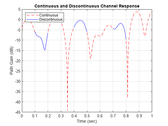
Plot the path gains for the continuous and discontinuous cases. The results show that the gains for the three segments match the gain for the continuous case. The alignment of the two shows that the sum-of-sinusoids technique is ideally suited to the simulation of packetized data because the channel characteristics are maintained even when data is not transmitted.
plot(t0,pathGain0,'r--')
hold on
plot(t1,pathGain1,'b')
plot(t2,pathGain2,'b')
plot(t3,pathGain3,'b')
grid
title('Continuous and Discontinuous Channel Response')
xlabel('Time (sec)')
ylabel('Path Gain (dB)')
legend('Continuous','Discontinuous','location','nw')
Input Arguments
Output Arguments
Version History
Introduced in R2012a