qamdemod

Quadrature amplitude demodulation

Syntax

Z = qamdemod(Y,M)

Z = qamdemod(Y,M,symOrder)

Z = qamdemod(___,Name=Value)

Description

Z = qamdemod(Y,M) returns a demodulated signal, Z, given quadrature amplitude modulation (QAM) signal Y of modulation order M.

example

Z = qamdemod(Y,M,symOrder) returns a demodulated signal, Z, and specifies the symbol order for the demodulation.

example

Z = qamdemod(___,Name=Value) specifies options using one or more name-value arguments. For example, OutputType=bit sets the type of output signal to bits.

example

Examples

collapse all

Demodulate 8-QAM Signal

Open Live Script

Demodulate an 8-QAM signal and plot the points corresponding to symbols 0 and 3.

Generate random 8-ary data symbols.

data = randi([0 7],1000,1);

Modulate data by applying 8-QAM.

txSig = qammod(data,8);

Pass the modulated signal through an AWGN channel.

rxSig = awgn(txSig,18,'measured');

Demodulate the received signal using an initial phase of $π$ /8.

rxData = qamdemod(rxSig.*exp(-1i*pi/8),8);

Generate the reference constellation points.

refpts = qammod((0:7)',8) .* exp(1i*pi/8);

Plot the received signal points corresponding to symbols 0 and 3 and overlay the reference constellation. The received data corresponding to those symbols is displayed.

plot(rxSig(rxData==0),'g.');
hold on
plot(rxSig(rxData==3),'c.');
plot(refpts,'r*')
text(real(refpts)+0.1,imag(refpts),num2str((0:7)'))
xlabel('In-Phase')
ylabel('Quadrature')
legend('Points corresponding to 0','Points corresponding to 3', ...
    'Reference constellation','location','nw');

Figure contains an axes object. The axes object with xlabel In-Phase, ylabel Quadrature contains 11 objects of type line, text. One or more of the lines displays its values using only markers These objects represent Points corresponding to 0, Points corresponding to 3, Reference constellation.

QAM Demodulation with WLAN Symbol Mapping

Open Live Script

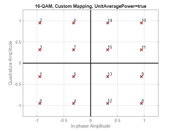
Modulate and demodulate random data by using 16-QAM with WLAN symbol mapping. Verify that the input data symbols match the demodulated symbols.

Generate a 3-D array of random symbols.

x = randi([0,15],20,4,2);

Create a custom symbol mapping for the 16-QAM constellation based on WLAN standards.

wlanSymMap = [2 3 1 0 6 7 5 4 14 15 13 12 10 11 9 8];

Modulate the data, and set the constellation to have unit average signal power. Plot the constellation.

y = qammod(x,16,wlanSymMap, ...
    UnitAveragePower=true, ...
    PlotConstellation=true);

Figure contains an axes object. The axes object with title 16-QAM, Custom Mapping, UnitAveragePower=true, xlabel In-phase Amplitude, ylabel Quadrature Amplitude contains 19 objects of type line, text. One or more of the lines displays its values using only markers

Demodulate the received signal.

z = qamdemod(y,16,wlanSymMap, ...
    UnitAveragePower=true);

Verify that the demodulated signal is equal to the original data.

isequal(x,z)

ans = logical
   1

Demodulate QAM Fixed-Point Signal

Open Live Script

Demodulate a fixed-point QAM signal and verify that the data is recovered correctly.

Set the modulation order as 64, and determine the number of bits per symbol.

M = 64;
bitsPerSym = log2(M);

Generate random bits. When operating in bit mode, the length of the input data must be an integer multiple of the number of bits per symbol.

x = randi([0 1],10*bitsPerSym,1);

Modulate the input data using a binary symbol mapping. Set the modulator to output fixed-point data. The numeric data type is signed with a 16-bit word length and a 10-bit fraction length.

y = qammod(x,M,'bin', ...
    InputType='bit', ...
    OutputDataType=numerictype(1,16,10));

Demodulate the 64-QAM signal. Verify that the demodulated data matches the input data.

z = qamdemod(y,M,'bin',OutputType='bit');
s = isequal(x,double(z))

s = logical
   1

Estimate BER for Hard and Soft Decision Viterbi Decoding

Open Live Script

Estimate bit error rate (BER) performance for hard-decision and soft-decision Viterbi decoders in AWGN. Compare the performance to that of an uncoded 64-QAM link.

Set the simulation parameters.

rng default
M = 64;                % Modulation order
k = log2(M);           % Bits per symbol
EbNoVec = (4:10)';     % Eb/No values (dB)
numSymPerFrame = 1000; % Number of QAM symbols per frame

Initialize the BER results vectors.

berEstSoft = zeros(size(EbNoVec)); 
berEstHard = zeros(size(EbNoVec));

Set the trellis structure and traceback depth for a rate 1/2, constraint length 7, convolutional code.

trellis = poly2trellis(7,[171 133]);
tbl = 32;
rate = 1/2;

The main processing loops perform these steps:

Generate binary data
Convolutionally encode the data
Apply QAM modulation to the data symbols. Specify unit average power for the transmitted signal
Pass the modulated signal through an AWGN channel
Demodulate the received signal using hard decision and approximate LLR methods. Specify unit average power for the received signal
Viterbi decode the signals using hard and unquantized methods
Calculate the number of bit errors

The while loop continues to process data until either 100 errors are encountered or $10^{7}$ bits are transmitted.

for n = 1:length(EbNoVec)
    % Convert Eb/No to SNR
    snrdB = EbNoVec(n) + 10*log10(k*rate);
    % Noise variance calculation for unity average signal power
    noiseVar = 10.^(-snrdB/10);
    % Reset the error and bit counters
    [numErrsSoft,numErrsHard,numBits] = deal(0);
    
    while numErrsSoft < 100 && numBits < 1e7
        % Generate binary data and convert to symbols
        dataIn = randi([0 1],numSymPerFrame*k,1);
        
        % Convolutionally encode the data
        dataEnc = convenc(dataIn,trellis);
        
        % QAM modulate
        txSig = qammod(dataEnc,M, ...
            InputType='bit', ...
            UnitAveragePower=true);
        
        % Pass through AWGN channel
        rxSig = awgn(txSig,snrdB,'measured');
        
        % Demodulate the noisy signal using hard decision (bit) and
        % soft decision (approximate LLR) approaches.
        rxDataHard = qamdemod(rxSig,M, ...
            OutputType='bit', ...
            UnitAveragePower=true);
        rxDataSoft = qamdemod(rxSig,M, ...
            OutputType='approxllr', ...
            UnitAveragePower=true, ...
            NoiseVariance=noiseVar);
        
        % Viterbi decode the demodulated data
        dataHard = vitdec(rxDataHard,trellis,tbl,'cont','hard');
        dataSoft = vitdec(rxDataSoft,trellis,tbl,'cont','unquant');
        
        % Calculate the number of bit errors in the frame. 
        % Adjust for the decoding delay, which is equal to 
        % the traceback depth.
        numErrsInFrameHard = ...
            biterr(dataIn(1:end-tbl),dataHard(tbl+1:end));
        numErrsInFrameSoft = ...
            biterr(dataIn(1:end-tbl),dataSoft(tbl+1:end));
        
        % Increment the error and bit counters
        numErrsHard = numErrsHard + numErrsInFrameHard;
        numErrsSoft = numErrsSoft + numErrsInFrameSoft;
        numBits = numBits + numSymPerFrame*k;

    end
    
    % Estimate the BER for both methods
    berEstSoft(n) = numErrsSoft/numBits;
    berEstHard(n) = numErrsHard/numBits;
end

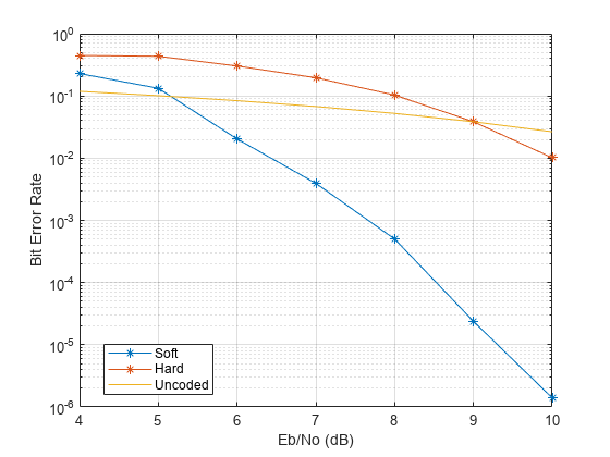
Plot the estimated hard and soft BER data. Plot the theoretical performance for an uncoded 64-QAM channel.

semilogy(EbNoVec,[berEstSoft berEstHard],'-*')
hold on
semilogy(EbNoVec,berawgn(EbNoVec,'qam',M))
legend('Soft','Hard','Uncoded','location','best')
grid
xlabel('Eb/No (dB)')
ylabel('Bit Error Rate')

Figure contains an axes object. The axes object with xlabel Eb/No (dB), ylabel Bit Error Rate contains 3 objects of type line. These objects represent Soft, Hard, Uncoded.

As expected, the soft decision decoding produces the best results.

Soft-Decision OQPSK Modulation-Demodulation

Open Live Script

Use the qamdemod function to simulate soft decision output for OQPSK-modulated signals.

Generate an OQPSK modulated signal.

sps = 4;
msg = randi([0 1],1000,1);
oqpskMod = comm.OQPSKModulator( ...
    SamplesPerSymbol=sps, ...
    BitInput=true);
oqpskSig = oqpskMod(msg);

Add noise to the generated signal.

impairedSig = awgn(oqpskSig,15);

Perform Soft-Decision Demodulation

Create QPSK equivalent signal to align in-phase and quadrature.

impairedQPSK = complex( ...
    real(impairedSig(1+sps/2:end-sps/2)), ...
    imag(impairedSig(sps+1:end)));

Apply matched filtering to the received OQPSK signal.

halfSinePulse = sin(0:pi/sps:(sps)*pi/sps);
matchedFilter = dsp.FIRDecimator(sps,halfSinePulse, ...
    DecimationOffset=sps/2);
filteredQPSK = matchedFilter(impairedQPSK);

To perform soft demodulation of the filtered OQPSK signal use the qamdemod function. Align symbol mapping of qamdemod with the symbol mapping used by the comm.OQPSKModulator, then demodulate the signal.

oqpskModSymbolMapping = [1 3 0 2];
demodulated = qamdemod(filteredQPSK,4,oqpskModSymbolMapping, ...
    OutputType='llr');

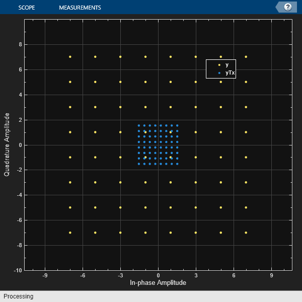
Average Power Normalization for QAM

Open Live Script

Apply average power normalization for hard decision output when using qammod and qamdemod functions by using the helperAvgPow2MinD utility function. Scale the constellation to the normalized average power, and then plot the reference and scaled constellations.

Compute the minimum distance for symbols based on specified average power and modulation order.

M = 64;
avgPwr = 2;
minD = helperAvgPow2MinD(avgPwr,M);

Modulate a signal composed of random integers in the range [0, M - 1], scale the modulated symbols.

x = randi([0,M-1],1000,1);
y = qammod(x,M);
yTx = (minD/2) .* y;

Verify signal average power approximately equals the specified average power, avgPow.

sigPwr = mean(abs(yTx).^2)

sigPwr = 
2.0141

avgPwr

avgPwr = 
2

Assign the transmitted signal to the receive signal without applying any RF or channel impairments. With no impairments to distort the received signal, the demodulated matches the original signal. Demodulate symbols using hard decisions, and confirm correct signal demodulation.

yRx = yTx;
z = qamdemod(yRx*2/minD,M);
checkDemodIsEqual = isequal(x,z)

checkDemodIsEqual = logical
   1

refC = qammod([0:M-1]',M);

Show constellation

maxAx = ceil(max(abs(refC)));
cd = comm.ConstellationDiagram(2, ...
    'ShowReferenceConstellation',0, ...
    'ShowLegend',true, ...
    'XLimits',[-(maxAx) maxAx],'YLimits',[-(maxAx) maxAx], ...
    'ChannelNames', ...
    {'y','yTx'});
cd(y,yTx)

Peak Power Normalization for QAM

Open Live Script

Apply peak power normalization for hard decision output when using qammod and qamdemod functions by using the helperPeakPow2MinD utility function. Scale the constellation to the normalized peak power, and then plot the reference and scaled constellations.

Compute the minimum distance for symbols based on specified peak power and modulation order.

M = 16;
pkPwr = 30;
minD = helperPeakPow2MinD(pkPwr,M);

Modulate a signal composed of random integers in the range [0, M - 1], scale the modulated symbols.

x = randi([0,M-1],1000,1);
y = qammod(x,M);
yTx = (minD/2) .* y;

Verify signal peak power approximately equals the specified peak power, pkPow.

sigPwr = max(abs(yTx).^2)

sigPwr = 
30

pkPwr

pkPwr = 
30

yRx = yTx;
z = qamdemod(yRx*2/minD,M);
checkDemodIsEqual = isequal(x,z)

checkDemodIsEqual = logical
   1

refC = qammod([0:M-1]',M);

Show constellation

maxAx = ceil(max(abs(refC)));
cd = comm.ConstellationDiagram(2, ...
    'ShowReferenceConstellation',0, ...
    'ShowLegend',true, ...
    'XLimits',[-(maxAx) maxAx],'YLimits',[-(maxAx) maxAx], ...
    'ChannelNames', ...
    {'y','yTx'});
cd(y,yTx)

Input Arguments

collapse all

`Y` — Input signal
scalar | vector | matrix | 3-D array

Input signal that resulted QAM, specified as a scalar, vector, matrix, or 3-D array of complex values. Each column in the matrix and 3-D array is considered as an independent channel.

Data Types: double | single | fi
Complex Number Support: Yes

`M` — Modulation order
positive integer power of two

Modulation order, specified as a positive integer power of two. The modulation order specifies the number of points in the signal constellation.

`symOrder` — Symbol order
`'gray'` (default) | `'bin'` | vector

Symbol order, specified as one of these options:

'gray' — Use Gray-coded ordering. For more information, see Gray Code.
'bin' — Use binary-coded ordering.
Vector — Use custom symbol ordering. The vector must be of length M. Vectors must use unique elements values in the range [0, (M – 1)]. The first element corresponds to the upper left point of the constellation, with subsequent elements running down column-wise from left to right.

Name-Value Arguments

Specify optional pairs of arguments as Name1=Value1,...,NameN=ValueN, where Name is the argument name and Value is the corresponding value. Name-value arguments must appear after other arguments, but the order of the pairs does not matter.

Before R2021a, use commas to separate each name and value, and enclose Name in quotes.

Example: Z = qamdemod(Y,M,symOrder,'OutputType','bit')

`UnitAveragePower` — Option to scale constellation to unit average power
`false` or `0` (default) | `true` or `1`

Option to scale constellation to unit average power, specified as a numeric or logical 0 (false) or 1 (true).

When set to true, the function scales the constellation to the average power of one watt referenced to 1 ohm.
When set to false, the function scales the constellation so that the QAM constellation points are separated by a minimum distance of two.

`OutputType` — Type of output
`'integer'` (default) | `'bit'` | `'llr'` | `'approxllr'`

Type of output, specified as 'integer', 'bit', 'llr', or 'approxllr'.

`OutputDataType` — Output data type
`'double'` | `'single'` | `'uint8'` | `'uint16'` | `'uint32'` | `'int8'` | `'int16'` | `'int32'` | `'logical'`

Output data type, specified as 'double', 'single', 'uint8' , 'uint16', 'uint32', 'int8''int16', 'int32', or 'logical'. This argument determines the final data type of the output modulated symbols.

When you specify OutputType as 'integer'or 'bit', you can specify the output data type as 'double', 'single', 'uint8', 'uint16', 'uint32', 'int8' 'int16', or 'int32'.
When you specify OutputType as 'bit', you can also specify the output data type as 'logical'.
When you specify OutputType as 'llr' or 'approxllr', this argument is ignored and the output data type is same as the data type of input Y.
If you do not specify this argument, the output data type is same as the data type of input Y for floating point Y and uint1 for fixed-point Y.

`NoiseVariance` — Noise variance
`1` (default) | positive scalar | vector of positive values

Noise variance, specified as a positive scalar or a vector of positive values. When you set this argument to a:

Positive scalar — The same noise variance value is used on all input elements.
Vector of positive values — The vector length must be equal to the number of elements in the last dimension of the input signal. Each element of the vector specifies the noise variance for all the elements of the input along the corresponding last dimension.

Tips

The exact LLR algorithm computes exponentials using finite precision arithmetic. For computations involving very large positive or negative magnitudes, the exact LLR algorithm yields:

Inf or -Inf if the noise variance is a very large value
NaN if the noise variance and signal power are both very small values

The approximate LLR algorithm does not compute exponentials. You can avoid Inf, -Inf, and NaN results by using the approximate LLR algorithm.

Dependencies

To enable this name-value pair argument, set OutputType is 'llr' or 'approxllr'.

`PlotConstellation` — Option to plot constellation
`false` or `0` (default) | `true` or `1`

Option to plot constellation, specified as a numeric or logical 0 (false) or 1 (true) To plot the QAM constellation, specify PlotConstellation=true.

Output Arguments

collapse all

`Z` — Demodulated output signal
scalar | vector | matrix | 3-D array

Demodulated output signal, returned as a scalar, vector, matrix, or 3-D array. The data type is the same as that of the input signal, Y. The value and dimension of this output vary depending on the specified OutputType value, as shown in this table.

`'OutputType'`	Return Value of `qamdemod`	Dimensions of Output
`'integer'`	Demodulated integer values in the range [0, (`M` – 1)]	`Z` has the same dimensions as input `Y`.
`'bit'`	Demodulated bits	The number of rows in `Z` is log₂(`M`) times the number of rows in `Y`. Each demodulated symbol is mapped to a group of log₂(`M`) bits, where the first bit represents the most significant bit (MSB) and the last bit represents the least significant bit (LSB).
`'llr'`	Log-likelihood ratio value for each bit calculated using the Exact Log Likelihood algorithm. For more details, see Exact LLR Algorithm.
`'approxllr'`	Approximate log-likelihood ratio value for each bit. The values are calculated using the Approximate Log Likelihood algorithm. For more details, see Approximate LLR Algorithm.

More About

collapse all

Gray Code

A Gray code, also known as a reflected binary code, is a system where the bit patterns in adjacent constellation points differ by only one bit.

Extended Capabilities

C/C++ Code Generation
Generate C and C++ code using MATLAB® Coder™.

GPU Arrays
Accelerate code by running on a graphics processing unit (GPU) using Parallel Computing Toolbox™.

This function supports GPU array inputs. For more information, see Run MATLAB Functions on a GPU (Parallel Computing Toolbox).

Version History

Introduced before R2006a

expand all

R2024a: Enhance output data type support

The qamdemod function enhances output data type offering by using the OutputDataType argument. Previously, the output data type was inherited from input data type or set to a fixed-point setting. This addition allows you to also specify the output data type as single or double.

R2023b: Add GPU array support

The qamdemod function adds support for gpuArray (Parallel Computing Toolbox) object processing to run code on a graphics processing unit (GPU).

R2018b: Initial Phase Input Removed

Starting in R2018b, you can no longer offset the initial phase for the QAM constellation using the qamdemod function.

Instead, use the genqamdemod function to offset the initial phase of the QAM signal being demodulated. Alternatively, you can multiply the modulated input of qamdemod by the desired initial phase, as shown in this code

Z = qamdemod(Y.*exp(-1i*initPhase,M))

qamdemod

Syntax

Description

Examples

Demodulate 8-QAM Signal

QAM Demodulation with WLAN Symbol Mapping

Demodulate QAM Fixed-Point Signal

Estimate BER for Hard and Soft Decision Viterbi Decoding

Soft-Decision OQPSK Modulation-Demodulation

Average Power Normalization for QAM

Peak Power Normalization for QAM

Input Arguments

`Y` — Input signal
scalar | vector | matrix | 3-D array

`M` — Modulation order
positive integer power of two

`symOrder` — Symbol order
`'gray'` (default) | `'bin'` | vector

Name-Value Arguments

`UnitAveragePower` — Option to scale constellation to unit average power
`false` or `0` (default) | `true` or `1`

`OutputType` — Type of output
`'integer'` (default) | `'bit'` | `'llr'` | `'approxllr'`

`OutputDataType` — Output data type
`'double'` | `'single'` | `'uint8'` | `'uint16'` | `'uint32'` | `'int8'` | `'int16'` | `'int32'` | `'logical'`

`NoiseVariance` — Noise variance
`1` (default) | positive scalar | vector of positive values

Tips

Dependencies

`PlotConstellation` — Option to plot constellation
`false` or `0` (default) | `true` or `1`

Output Arguments

`Z` — Demodulated output signal
scalar | vector | matrix | 3-D array

More About

Gray Code

Extended Capabilities

C/C++ Code Generation
Generate C and C++ code using MATLAB® Coder™.

GPU Arrays
Accelerate code by running on a graphics processing unit (GPU) using Parallel Computing Toolbox™.

Version History

R2024a: Enhance output data type support

R2023b: Add GPU array support

R2018b: Initial Phase Input Removed

See Also

Functions

Topics

qamdemod

Syntax

Description

Examples

Demodulate 8-QAM Signal

QAM Demodulation with WLAN Symbol Mapping

Demodulate QAM Fixed-Point Signal

Estimate BER for Hard and Soft Decision Viterbi Decoding

Soft-Decision OQPSK Modulation-Demodulation

Average Power Normalization for QAM

Peak Power Normalization for QAM

Input Arguments

Y — Input signal scalar | vector | matrix | 3-D array

M — Modulation order positive integer power of two

symOrder — Symbol order 'gray' (default) | 'bin' | vector

Name-Value Arguments

UnitAveragePower — Option to scale constellation to unit average power false or 0 (default) | true or 1

OutputType — Type of output 'integer' (default) | 'bit' | 'llr' | 'approxllr'

OutputDataType — Output data type 'double' | 'single' | 'uint8' | 'uint16' | 'uint32' | 'int8' | 'int16' | 'int32' | 'logical'

NoiseVariance — Noise variance 1 (default) | positive scalar | vector of positive values

Tips

Dependencies

PlotConstellation — Option to plot constellation false or 0 (default) | true or 1

Output Arguments

Z — Demodulated output signal scalar | vector | matrix | 3-D array

More About

Gray Code

Extended Capabilities

C/C++ Code Generation Generate C and C++ code using MATLAB® Coder™.

GPU Arrays Accelerate code by running on a graphics processing unit (GPU) using Parallel Computing Toolbox™.

Version History

R2024a: Enhance output data type support

R2023b: Add GPU array support

R2018b: Initial Phase Input Removed

See Also

Functions

Topics

`Y` — Input signal
scalar | vector | matrix | 3-D array

`M` — Modulation order
positive integer power of two

`symOrder` — Symbol order
`'gray'` (default) | `'bin'` | vector

`UnitAveragePower` — Option to scale constellation to unit average power
`false` or `0` (default) | `true` or `1`

`OutputType` — Type of output
`'integer'` (default) | `'bit'` | `'llr'` | `'approxllr'`

`OutputDataType` — Output data type
`'double'` | `'single'` | `'uint8'` | `'uint16'` | `'uint32'` | `'int8'` | `'int16'` | `'int32'` | `'logical'`

`NoiseVariance` — Noise variance
`1` (default) | positive scalar | vector of positive values

`PlotConstellation` — Option to plot constellation
`false` or `0` (default) | `true` or `1`

`Z` — Demodulated output signal
scalar | vector | matrix | 3-D array

C/C++ Code Generation
Generate C and C++ code using MATLAB® Coder™.

GPU Arrays
Accelerate code by running on a graphics processing unit (GPU) using Parallel Computing Toolbox™.