assemble

Assemble components by connecting their physical interfaces

Since R2026a

collapse all in page

Syntax

sysCon = assemble(sys1,sys2,Port1,Port2)

sysCon = assemble(sys1,sys2,Port1,Port2,Ki,Ci)

sysCon = assemble(sys1,sys2,Port1,Port2,Qi)

sysCon = assemble(S,Port1,Port2,___)

sysCon = assemble(___,Method=assemblyMethod)

Description

Use the assemble function to assemble two components (parts) by adding some physical coupling at their interfaces (physical ports). The function supports rigid, compliant, and generalized couplings. You must first define the interfaces using the addInterface function

sysCon = assemble(sys1,sys2,Port1,Port2) adds a rigid coupling between the ports of the parts sys1 and sys2 identified by Port1 and Port2. Ports are designated by strings of the form sysName:PortName. To rigidly couple the port Port1 to the ground, set Port2 = "Ground".

sysCon = assemble(sys1,sys2,Port1,Port2,Ki,Ci) adds a compliant coupling between the ports of the parts sys identified by Port1 and Port2 . Ki is the coupling stiffness and Ci is the coupling damping. This corresponds to the internal force $λ = K_{i} δ + C_{i} \dot{δ}$ acting on Port1 with negative sign and Port2 with positive sign, where δ = z₁ – z₂ is the position mismatch between the coupled nodes. To add a compliant coupling between Port1 and the ground, set Port2 = "Ground".

example

sysCon = assemble(sys1,sys2,Port1,Port2,Qi) adds a generalized coupling λ = Q_i(s)δ between the ports of the parts sys identified by Port1 and Port2. To add a generalized coupling between Port1 and the ground, set Port2 = "Ground".

example

sysCon = assemble(S,Port1,Port2,___) adds coupling between the ports of the parts of uncoupled superstructure S identified by Port1 and Port2. Typically, you create such an uncoupled superstructure using append.

sysCon = assemble(___,Method=assemblyMethod) specifies the assembly method as "primal" or "dual". The default is "dual". You use primal models only when most rows of Hu and most columns of Hy are zero. Dense Hu or Hy can lead to substantial fill-in in the assembly model.

example

Examples

collapse all

Create Torsional Coupling Between Two Bodies Using Generalized Coupling of Components

Open Live Script

This example shows how to create a generalized coupling between two parts. For this example, you model a connection between inertia 1 and inertia 2 as a generalized torsional coupling. You can represent the system dynamics as follows.

$J_{1} {θ_{}^{¨}}_{1} = T_{1} - T_{c}$

$J_{2} {θ_{}^{¨}}_{2} = T_{2} + T_{c}$

$J_{c} ({θ_{}^{¨}}_{1} - {θ_{}^{¨}}_{2}) + b_{c} ({θ_{}^{˙}}_{1} - {θ_{}^{˙}}_{2}) + k_{c} (θ_{1} - θ_{2}) = T_{c}$

Here:

$J_{1}$ and $J_{2}$ is the inertia of body 1 and 2, respectively.
$θ_{1}$ and $θ_{2}$ is the angular positions of body 1 and 2, respectively.
$T_{1}$ is the input torque and $T_{2}$ is the load torque.
$T_{c}$ is the coupling torque.
$J_{c}$ is the coupling inertia.
$k_{c}$ is the coupling stiffness.
$b_{c}$ is the coupling damping.

Define the model parameters.

J1 = 2;      % kg*m^2
J2 = 1;      % kg*m^2
Jc = 0.1;    % kg*m^2
bc = 0.1;    % N*m*s/rad
kc = 10;     % N*m/rad

Assembly of Individual Components

addInterface augments the inputs and outputs of the model to include the displacements as extra outputs and forces as extra inputs associated with a particular coupling interface.

$\begin{array}{l} E x_{}^{˙} = A x + B u + H_{u} λ \\ y = C x \\ z = H_{y} x \end{array}$

These coupling dynamics model the action-reaction reaction forces $λ$ between two parts. When you use the assembly interface, the software automatically handles the force balance between the two components. For this example, inertia 1 exerts a torque $T_{c}$ on inertia 2, while inertia 2 exerts a torque $- T_{c}$ on inertia 1. Therefore, you can define the individual dynamics and coupling as follows.

Inertia 1

$[\begin{array}{cc} 1 & 0 \\ 0 & J_{1} \end{array}] [\begin{array}{c} {θ_{}^{˙}}_{1} \\ {θ_{}^{¨}}_{1} \end{array}] = [\begin{array}{cc} 0 & 1 \\ 0 & 0 \end{array}] [\begin{array}{c} θ_{1} \\ {θ_{}^{˙}}_{1} \end{array}] + [\begin{array}{c} 0 \\ 1 \end{array}] T_{1} - \underset{H_{u 1} λ}{{[\begin{array}{c} 0 \\ 1 \end{array}] T_{c}}_{⏟}^{}}$

Inertia 2

$[\begin{array}{cc} 1 & 0 \\ 0 & J_{2} \end{array}] [\begin{array}{c} {θ_{}^{˙}}_{2} \\ {θ_{}^{¨}}_{2} \end{array}] = [\begin{array}{cc} 0 & 1 \\ 0 & 0 \end{array}] [\begin{array}{c} θ_{2} \\ {θ_{}^{˙}}_{2} \end{array}] + [\begin{array}{c} 0 \\ 1 \end{array}] T_{2} + \underset{H_{u 2} λ}{{[\begin{array}{c} 0 \\ 1 \end{array}] T_{c}}_{⏟}^{}}$

Coupling

$J_{c} ({θ_{}^{¨}}_{1} - {θ_{}^{¨}}_{2}) + b_{c} ({θ_{}^{˙}}_{1} - {θ_{}^{˙}}_{2}) + k_{c} (θ_{1} - θ_{2}) = T_{c}$

$T_{c} (s) = Q (s) (θ_{1} - θ_{2})$

$Q (s) = J_{c} s^{2} + b_{c} s + k_{c}$

When you assemble parts using a generalized coupling, the software models the coupling dynamics as $λ = Q (s) δ$ , where $λ$ is obtained as the output of linear system driven by the gap $δ = z_{1} - z_{2} = θ_{1} - θ_{2}$ .

Create the state-space model and define the interface for inertia 1.

E1 = [1 0; 0 J1];
A1 = [0 1; 0 0];
B1 = [0;1];
C1 = [0 1]; % output angular velocity w1
D1 = 0;
sys1 = dss(A1,B1,C1,D1,E1);
sys1.Name = "inertia1";
sys1.InputName = "Input Torque";
sys1.OutputName = "w1";
Hu1 = [0;1]; 
Hy1 = [1 0]; % z1 = theta1
sys1 = addInterface(sys1,"w1tow2",Hy1,Hu1)

sys1 =
 
  A = 
       x1  x2
   x1   0   1
   x2   0   0
 
  B = 
       Input Torque  inertia1:w1t
   x1             0             0
   x2             1             1
 
  C = 
                 x1  x2
   w1             0   1
   inertia1:w1t   1   0
 
  D = 
                 Input Torque  inertia1:w1t
   w1                       0             0
   inertia1:w1t             0             0
 
  E = 
       x1  x2
   x1   1   0
   x2   0   2
 
Input groups:                
        Name         Channels
   inertia1_w1tow2      2    
Output groups:               
        Name         Channels
   inertia1_w1tow2      2    
Name: inertia1
Continuous-time state-space model.
Model Properties

The addInterface function adds an extra input and output to facilitate the coupling at this interface.

Similarly, define the interface for inertia 2.

E2 = [1 0; 0 J2];
A2 = [0 1; 0 0];
B2 = [0;1];
C2 = [0 1]; % output angular velocity w1
D2 = 0;
sys2 = dss(A2,B2,C2,D2,E2);
sys2.Name = "inertia2";
sys2.InputName = "Load Torque";
sys2.OutputName = "w2";
Hu2 = [0;1];
Hy2 = [1 0]; % z2 = theta2
sys2 = addInterface(sys2,"w2tow1",Hy2,Hu2)

sys2 =
 
  A = 
       x1  x2
   x1   0   1
   x2   0   0
 
  B = 
        Load Torque  inertia2:w2t
   x1             0             0
   x2             1             1
 
  C = 
                 x1  x2
   w2             0   1
   inertia2:w2t   1   0
 
  D = 
                  Load Torque  inertia2:w2t
   w2                       0             0
   inertia2:w2t             0             0
 
  E = 
       x1  x2
   x1   1   0
   x2   0   1
 
Input groups:                
        Name         Channels
   inertia2_w2tow1      2    
Output groups:               
        Name         Channels
   inertia2_w2tow1      2    
Name: inertia2
Continuous-time state-space model.
Model Properties

Define the coupling and assemble the model components.

Q = tf([Jc bc kc],1);
asys = assemble(sys1,sys2,"inertia1:w1tow2","inertia2:w2tow1",Q,Method="primal");

Compare with Full Dynamics Model

You can represent the model that accounts for generalized torsional dynamics in the following state-space form.

$\begin{array}{l} [\begin{array}{cccc} 1 & 0 & 0 & 0 \\ 0 & 1 & 0 & 0 \\ 0 & 0 & J_{1} + J_{c} & - J_{c} \\ 0 & 0 & - J_{c} & J_{2} + J_{c} \end{array}] [\begin{array}{c} {θ_{}^{˙}}_{1} \\ {θ_{}^{˙}}_{2} \\ {θ_{}^{¨}}_{1} \\ {θ_{}^{¨}}_{2} \end{array}] = [\begin{array}{cccc} 0 & 0 & 1 & 0 \\ 0 & 0 & 0 & 1 \\ - k_{c} & k_{c} & - b_{c} & b_{c} \\ k_{c} & - k_{c} & b_{c} & - b_{c} \end{array}] [\begin{array}{c} θ_{1} \\ θ_{2} \\ {θ_{}^{˙}}_{1} \\ {θ_{}^{˙}}_{2} \end{array}] + [\begin{array}{cc} 0 & 0 \\ 0 & 0 \\ 1 & 0 \\ 0 & 1 \end{array}] [\begin{array}{c} T_{1} \\ T_{2} \end{array}] \\ y = [\begin{array}{cccc} 0 & 0 & 1 & 0 \\ 0 & 0 & 0 & 1 \end{array}] [\begin{array}{c} θ_{1} \\ θ_{2} \\ {θ_{}^{˙}}_{1} \\ {θ_{}^{˙}}_{2} \end{array}] \end{array}$

Define the state-space matrices and create the model.

Ec = [ 1  0   0    0;
      0  1    0    0;
      0  0  J1+Jc  -Jc;
      0  0   -Jc   J2+Jc ];

Ac = [ 0  0   1    0;
      0  0   0    1;
    -kc kc -bc  bc;
     kc -kc  bc -bc ];

Bc = [ 0  0;
      0  0;
      1  0;
      0  1 ];
Cc = [0 0 1 0;
    0 0 0 1];
Dc = 0;
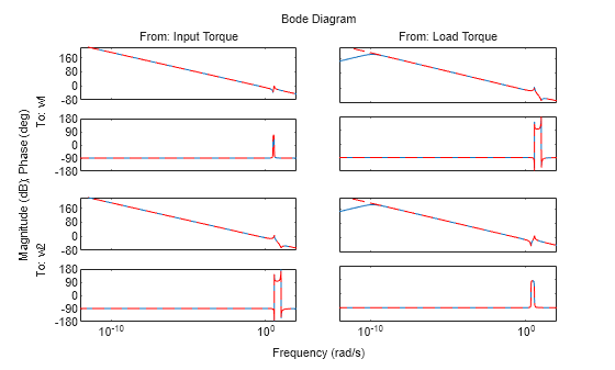
sysc = dss(Ac, Bc, Cc, Dc,Ec);

Comparing the Bode response of both models, you can see they are equivalent.

opt = bodeoptions;
opt.PhaseWrapping = "on";
bodeplot(asys,sysc,"r--",opt)

MATLAB figure

Simulate both models to a sinusoidal torque $T_{1}$ applied to inertia 1 and zero load torque $T_{2}$ .

t = 0:0.01:15;
u = [sin(t); zeros(size(t))];
ya = lsim(asys,u',t);
yc = lsim(sysc,u',t);
tiledlayout(2,1)
nexttile
plot(t,ya(:,1),t,yc(:,1),'r--');
title("\omega_1")
nexttile
plot(t,ya(:,2),t,yc(:,2),'r--');
title("\omega_2")
legend("Assembled model","Complete model")

Figure contains 2 axes objects. Axes object 1 with title omega indexOf 1 baseline contains 2 objects of type line. Axes object 2 with title omega indexOf 2 baseline contains 2 objects of type line. These objects represent Assembled model, Complete model.

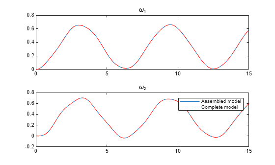
You can see that both approaches result in an equivalent model. Assembly of individual components is helpful when you want to couple several parts with some coupling dynamics.

Create Mass-Spring-Damper Model Using Compliant Coupling

Open Live Script

This example shows how to create a mass-spring-damper model using compliant coupling between a mass and a wall.

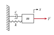
You can model this equation by:

$m x_{}^{¨} = F - F_{c}$

$x_{}^{¨} = \frac{1}{m} F + \frac{1}{m} (- F_{c})$

In this coupling, the mass exerts a force $F_{c}$ on the wall, while the wall exerts a force $- F_{c}$ on the mass. Modeling the mass and coupling dynamics separately, you get:

$\begin{array}{l} x_{}^{¨} = \frac{1}{m} F + \underset{H_{u} λ}{{\frac{1}{m} (- F_{c})}_{⏟}^{}} \\ y = x \\ z_{1} = x \end{array}$

$λ = (k (z_{1} - z_{2}) - b ({z_{1}}_{}^{˙} - {z_{}^{˙}}_{2}))$

Since the mass is connected to a wall (ground), $z_{2} = 0$ .

Define the model parameters.

m = 3;
c = 1;
k = 2;

Create the state-space model and define the coupling interface.

A = [0 1; 0 0];
B = [0; 1/m];
C = [1 0];
D = 0;
Hy = [1 0];
Hu = [0; 1/m];
sys = ss(A,B,C,D);
sys.Name = "mass";
sys.InputName = "force";
sys.OutputName = "displacement";
isys = addInterface(sys,"masstowall",Hy,Hu);

Since the mass is connected to a wall, connect the coupling interface port to the ground to create the assembled model.

asys = assemble(isys,"mass:masstowall","Ground",k,c);

Compare with Complete Model

The equation of motion that accounts for full dynamics is given by:

$m x_{}^{¨} = F - k x - c x_{}^{˙}$

Create the state-space model.

Ac = [0 1; -k/m -c/m];
Bc = [0;1/m];
Cc = [1 0];
Dc = 0;
sysc = ss(Ac,Bc,Cc,Dc);

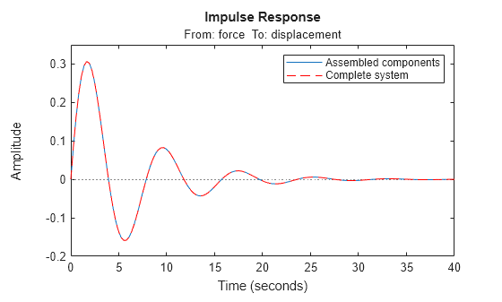
Simulating the impulse response of both models, you can see they are equivalent.

impulseplot(asys,sysc,"r--")
legend("Assembled components","Complete system")

MATLAB figure

Create Motor-Load-Shaft System with Gear Ratio and Compliant Coupling

Open Live Script

This example shows how to couple a motor and a load using compliant coupling. The and motor and load are connected by a gearbox, with coupling stiffness $k_{c}$ and gear ratio $N$ .

You can define the equations for this system as follows:

$J_{m} {θ_{m}}_{}^{¨} = T_{in} - T_{c}$

$J_{l} {θ_{l}}_{}^{¨} = \frac{1}{N} T_{c} - T_{l o a d}$

$T_{c} = k_{c} (θ_{m} - N θ_{l})$

Here:

$J_{m}$ is the motor inertia
$J_{l}$ is the load inertia
$T_{c}$ is the coupling torque
$k_{c}$ is the coupling stiffness
$N$ is the gear ratio, where motor rotates $N$ times faster than the load side
$θ_{m}$ is the motor shaft angle
$θ_{l}$ is the load shaft angle

Define the model parameters

Jm = 0.01;      % kg*m^2
Jl = 0.05;      % kg*m^2
kc = 10;        % N*m/rad
N  = 2;         % Gear ratio

Assembly of Individual Components

When you model this as an internal coupling, you can define the equations as follows.

${θ_{}^{¨}}_{m} = \frac{1}{J_{m}} T_{i n} - \underset{H_{u 1} λ}{{\frac{1}{J_{m}} (T_{c})}_{⏟}^{}}$

${θ_{}^{¨}}_{l} = \underset{H_{u 2} λ}{{\frac{1}{J_{l} N} (T_{c})}_{⏟}^{}} - \frac{1}{J_{l}} T_{l o a d}$

Here, $T_{c} = λ = k_{c} δ$ and the collocation gap $δ = z_{1} - z_{2}$ is defined relative to the state values, with $z_{1} = θ_{m}$ and $z_{2} = N θ_{l}$ .

Create the state-space model and define the coupling interface on the motor side.

Am = [0 1; 0 0];
Bm = [0; 1/Jm];
Cm = [1 0];
Dm = 0;
Hu1 = [0;1/Jm];
Hy1 = [1 0];   % z1 = theta_m
sysm = ss(Am,Bm,Cm,Dm);
sysm.Name = "motor";
sysm.InputName = "Input Torque";
sysm.OutputName = "Motor speed";
sysma = addInterface(sysm,"motortoload",Hy1,Hu1);

Similarly, define the coupling interface on the load side.

Al = [0 1; 0 0];
Bl = [0; -1/Jl];
Cl = [1 0];
Dl = 0;
Hu2 = [0;1/(Jl*N)];
Hy2 = [N 0];    % z2 = N*theta_l
sysl = ss(Al,Bl,Cl,Dl);
sysl.Name = "load";
sysl.InputName = "Load Torque";
sysl.OutputName = "Load speed";
sysla = addInterface(sysl,"loadtomotor",Hy2,Hu2);

Create the model assembly with compliant coupling with stiffness K = $k_{c}$ . When you do not specify a value for damping C, the software uses C = 0.

asys = assemble(sysma,sysla,"motor:motortoload","load:loadtomotor",kc);

Complete Model with Full Dynamics

You can define the model that accounts for full coupling dynamics in the state-space form as follows.

$\begin{array}{l} x_{}^{˙} = [\begin{array}{cccc} 0 & 1 & 0 & 0 \\ - \frac{k_{c}}{J_{m}} & 0 & \frac{k_{c} N}{J_{m}} & 0 \\ 0 & 0 & 0 & 1 \\ \frac{k_{c}}{J_{l} N} & 0 & - \frac{k_{c}}{J_{l}} & 0 \end{array}] [\begin{array}{c} θ_{m} \\ {θ_{}^{˙}}_{m} \\ θ_{l} \\ {θ_{}^{˙}}_{l} \end{array}] + [\begin{array}{cc} 0 & 0 \\ \frac{1}{J_{m}} & 0 \\ 0 & 0 \\ 0 & - \frac{1}{J_{l}} \end{array}] \\ y = [\begin{array}{cccc} 1 & 0 & 0 & 0 \\ 0 & 0 & 1 & 0 \end{array}] [\begin{array}{c} θ_{m} \\ {θ_{}^{˙}}_{m} \\ θ_{l} \\ {θ_{}^{˙}}_{l} \end{array}] \end{array}$

Create the state-space model.

Ac = [ 0,      1,      0,       0;
     -kc/Jm,   0,  (kc*N)/Jm,   0;
      0,       0,      0,       1;
   kc/(N*Jl),  0,   -kc/Jl,     0 ];

Bc = [ 0,      0;
      1/Jm,    0;
      0,       0;
      0,     -1/Jl ];

Cc = [1 0 0 0;
      0 0 1 0];
Dc = 0;
sysc = ss(Ac, Bc, Cc, Dc);

Compare Models

Simulate both models to a sinusoidal input torque and zero load torque.

t = 0:0.001:15;
u = [sin(t); zeros(size(t))];
yc = lsim(sysc,u',t);
ya = lsim(asys,u',t);

Compute the torsional deflection $θ_{d} = θ_{m} - N θ_{l}$ and plot the results.

ya_def = ya(:,1)-N.*ya(:,2);
yc_def = yc(:,1)-N.*yc(:,2);
plot(t,ya_def,t,yc_def,'r--');
title("Torsional Deflection")

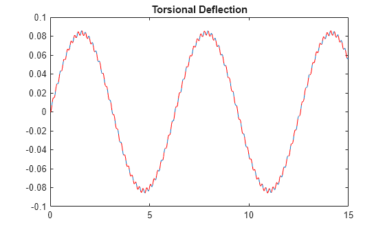
Figure contains an axes object. The axes object with title Torsional Deflection contains 2 objects of type line.

As you can see, both approaches result in an equivalent model. Notice the sustained oscillations in the torsional deflection. This the because there is no damping in the system.

Physical Connections Between Components in Sparse Second-Order Model

Open Live Script

For this example, consider a structural model that consists of two square plates connected with pillars at each vertex as depicted in the figure below. The lower plate is attached rigidly to the ground while the pillars are attached rigidly to each vertex of the square plate.

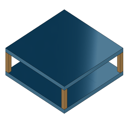
Load the finite element model matrices contained in platePillarModel.mat and create the sparse second-order model representing the above system.

load('platePillarModel.mat')

Define interfaces.

Plate1 = mechss(M1,[],K1,B1,F1,'Name','Plate1');
Plate2 = mechss(M2,[],K2,B2,F2,'Name','Plate2');

Now, load the interfaced degree of freedom (DOF) index data from dofData.mat and use interface to create the physical connections between the two plates and the four pillars. dofs is a 6x7 cell array where the first two rows contain DOF index data for the first and second plates while the remaining four rows contain index data for the four pillars. By default, the function uses dual-assembly method of physical coupling.

load('dofData.mat','dofs')
for ct=1:4
    % Plates to pillars
    Plate1 = addInterface(Plate1,"Pillar"+ct,dofs{1,2+ct});
    Plate2 = addInterface(Plate2,"Pillar"+ct,dofs{2,2+ct});
end

P = cell(4,1);
for ct=1:4
    % Pillars to plates
    P{ct} = mechss(Mp,[],Kp,Bp,Fp,'Name',"Pillar"+ct);
    P{ct} = addInterface(P{ct},"TopMount",dofs{2+ct,1});
    P{ct} = addInterface(P{ct},"BottomMount",dofs{2+ct,2});
end
% Plate 2 to ground

Specify connection between the bottom plate and the ground.

Plate2 = addInterface(Plate2,"Ground",dofs{2,7});

% Assemble
model = append(Plate1,Plate2,P{:});

Use showStateInfo to confirm the physical interfaces.

showStateInfo(model)

The state groups are:

    Type        Name      Size
  ----------------------------
  Component    Plate1     2646
  Component    Plate2     2646
  Component    Pillar1     132
  Component    Pillar2     132
  Component    Pillar3     132
  Component    Pillar4     132

sysConDual = model;
for ct=1:4
    sysConDual = assemble(sysConDual,"Plate1:Pillar"+ct,"Pillar"+ct+":TopMount"');
    sysConDual = assemble(sysConDual,"Plate2:Pillar"+ct,"Pillar"+ct+":BottomMount");
end
sysConDual = assemble(sysConDual,"Plate2:Ground","Ground");

Use showStateInfo to confirm the physical interfaces.

showStateInfo(sysConDual)

The state groups are:

    Type                      Name                   Size
  -------------------------------------------------------
  Component                  Plate1                  2646
  Component                  Plate2                  2646
  Component                 Pillar1                   132
  Component                 Pillar2                   132
  Component                 Pillar3                   132
  Component                 Pillar4                   132
  Interface     Plate1:Pillar1-Pillar1:TopMount        12
  Interface    Plate2:Pillar1-Pillar1:BottomMount      12
  Interface     Plate1:Pillar2-Pillar2:TopMount        12
  Interface    Plate2:Pillar2-Pillar2:BottomMount      12
  Interface     Plate1:Pillar3-Pillar3:TopMount        12
  Interface    Plate2:Pillar3-Pillar3:BottomMount      12
  Interface     Plate1:Pillar4-Pillar4:TopMount        12
  Interface    Plate2:Pillar4-Pillar4:BottomMount      12
  Interface           Plate2:Ground-Ground              6

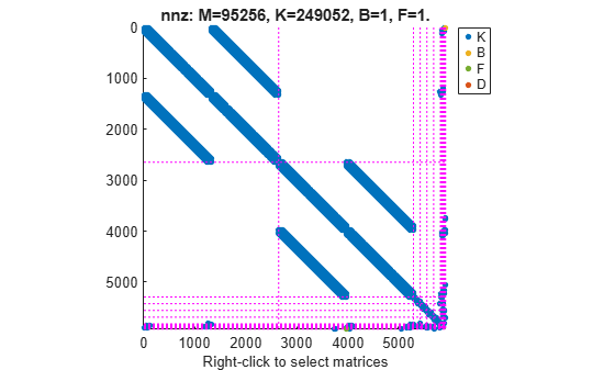
You can use spy to visualize the sparse matrices in the final model.

spy(sysConDual)

Figure contains an axes object. The axes object with title nnz: M=95256, K=249052, B=1, F=1., xlabel Right-click to select matrices contains 37 objects of type line. One or more of the lines displays its values using only markers These objects represent K, B, F, D.

Now, specify physical connections using the primal-assembly method.

sysConPrimal = model;
for ct=1:4
    sysConPrimal = assemble(sysConPrimal,"Plate1:Pillar"+ct,"Pillar"+ct+":TopMount"',Method="primal");
    sysConPrimal = assemble(sysConPrimal,"Plate2:Pillar"+ct,"Pillar"+ct+":BottomMount",Method="primal");
end
sysConPrimal = assemble(sysConPrimal,"Plate2:Ground","Ground",Method="primal");

Use showStateInfo to confirm the physical interfaces.

showStateInfo(sysConPrimal)

The state groups are:

    Type       Name    Size
  -------------------------
  Component            5718

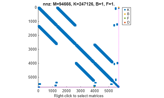
Primal assembly eliminates half of the redundant DOFs associated with the shared set of DOFs in the global finite element mesh.

You can use spy to visualize the sparse matrices in the final model.

spy(sysConPrimal)

Figure contains an axes object. The axes object with title nnz: M=94666, K=247126, B=1, F=1., xlabel Right-click to select matrices contains 9 objects of type line. One or more of the lines displays its values using only markers These objects represent K, B, F, D.

The data set for this example was provided by Victor Dolk from ASML.

Input Arguments

collapse all

`sys1`, `sys2` — Model with interfaces for coupling
`ss` object | `sparss` object | `mechss` object

Augmented system with interfaces defined using addInterface, specified as an ss, sparss, or mechss model object. The augmented model must contain:

Extra inputs for the forcing term f = H_uλ
Extra outputs for the displacements z = H_yx.
Input and output groups with name modelName_PortName.

`Port1`, `Port2` — Ports involved in physical coupling
string | `"Ground"`

Strings identifying the two ports involved in the physical coupling. The strings must be of the form "modelName:PortName". Additionally, if one of the ports is the ground, set the corresponding identifier to "Ground".

`Ki`, `Ci` — Stiffness and damping matrices
matrix

Stiffness and damping matrices, specified as square matrices of size n_i, where n_i is the number of couplings at the interface of sys.

`Qi` — Generalized coupling dynamics
dynamic system model

Generalized coupling dynamics, specified as a dynamic system model. Qi must have a valid ss representation and input-output dimensions must match the defined interface of sys. Additionally, Qi must be delay free.

`S` — Uncoupled superstructure
`ss` object | `sparss` object | `mechss` object

Uncoupled superstructure of multiple parts, specified as an ss, sparss, or mechss model object. This is equivalent to S = append(sys1,sys2).

`assemblyMethod` — Assembly method
`"dual"` (default) | `"primal"`

Interface assembly method, specified as one of the following:

"dual" — Use the dual-assembly method of physical coupling. This method maintains sparsity at the expense of additional algebraic variables.
"primal" — Use the primal-assembly method of physical coupling. This method uses a minimal number of DoFs but the system may suffer from fill-in.

For more information, see Algorithms.

Output Arguments

collapse all

`sysCon` — Assembled system
`ss` object | `sparss` object | `mechss` object

Assembled system, returned as a model of the same type as sys.

Algorithms

collapse all

In general, you can represent physical couplings in a block diagram form as shown in the following figure. The coupling is characterized by the "Coupling Dynamics" block mapping δ = z₁ − z₂ (collocation gap) to the internal forces λ. Here, z₁ and z₂ denote the positions on each part of the nodes being coupled together.

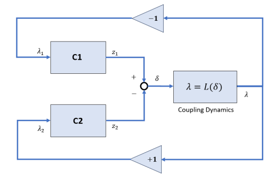
Using Control System Toolbox™, you can perform the following types of couplings between state-space models.

Rigid couplings, which correspond to δ = 0 and λ determined by the balance of forces. In this type of coupling, the positions, z₁ and z₂ match exactly (collocation) as if the two parts were welded together.
Compliant couplings, where $λ = K_{i} δ + C_{i} \dot{δ}$ . Here the coupling is modeled as a spring-damper connection and the two parts can move with respect to each other.
Generalized coupling, where λ = Q(s)δ. Here, you obtain λ as the output of a linear system driven by the gap δ. This can be used to model more complex coupling dynamics.

Rigid Coupling

Consider two components C₁ and C₂ described by:

$\begin{matrix} M_{1} {\ddot{q}}_{1} + K_{1} q_{1} = B_{1} u_{1}, & y_{1} = F_{1} q_{1} \\ M_{2} {\ddot{q}}_{2} + K_{2} q_{2} = B_{2} u_{2}, & y_{2} = F_{2} q_{2}, \end{matrix}$

with external I/Os u_j and y_j. The rigid coupling between C₁ and C₂ gives rise to two coupling conditions:

The collocation condition z₁ = z₂ where z₁ and z₂ are matching locations on C₁ and C₂ at the interface between the two components.
The balance of internal forces: C₁ exerts forces λ on C₂ at the locations z₂ while C₂ exerts forces –λ on C₁ at the locations z₁.

In the q₁, q₂ coordinates, you can express the locations z₁, z₂ as:

$\begin{matrix} z_{1} = H_{1} q_{1}, & z_{2} = H_{2} q_{2} \end{matrix},$

and capture the internal forces as additional inputs g₁, g₂ satisfying

$\begin{matrix} g_{1} = - H_{1}^{T} λ, & g_{2} = H_{2}^{T} λ \end{matrix} .$

This augments the C_j model with extra I/Os λ_j and z_j:

$\begin{array}{l} M_{j} {\ddot{q}}_{j} + K_{j} q_{j} = B_{j} u_{j} + g_{j} = B_{j} u_{j} + H_{j}^{T} λ \\ y_{j} = F_{j} q_{j} \\ \begin{matrix} z_{j} = H_{j} q_{j}, & j = 1, 2 \end{matrix} . \end{array}$

Hence, you can represent interfaces for physical couplings as extra inputs (coupling forces) and outputs (displacements at the interface).

For the augmented model C_j, the coupling equations are:

$\begin{matrix} z_{1} = z_{2}, & λ_{2} \end{matrix} = - λ_{1} = λ .$

Dual-Assembly Model

Combining all equations, you get the following model of the C₁ + C₂ assembly:

$\begin{array}{l} [\begin{matrix} M & 0 \\ 0 & 0 \end{matrix}] [\begin{matrix} \ddot{q} \\ \ddot{λ} \end{matrix}] + [\begin{matrix} K & H^{T} \\ H & 0 \end{matrix}] [\begin{matrix} q \\ λ \end{matrix}] = [\begin{matrix} B \\ 0 \end{matrix}] u \\ y = [\begin{matrix} F & 0 \end{matrix}] [\begin{matrix} q \\ λ \end{matrix}] \end{array}$

with

$\begin{matrix} q = [\begin{matrix} q_{1} \\ q_{2} \end{matrix}], & u = [\begin{matrix} u_{1} \\ u_{2} \end{matrix}], & y = [\begin{matrix} y_{1} \\ y_{2} \end{matrix}], & H = [\begin{matrix} H_{1} & - H_{2} \end{matrix}] \end{matrix} .$

Primal-Assembly Model

For rigid interfaces, primal assembly consists of eliminating half of the redundant DOFs associated with the following constraint.

$\begin{matrix} z_{1} = z_{2}, & λ_{2} \end{matrix} = - λ_{1} = λ .$

If Hq = 0 is the matrix expression of this constraint, this amounts to writing q = Lq_r. Here, q_r is the set of independent (free) DOFs and L spans the null space of H.

$H L = 0$

Using q = Lq_r, the equations

$\begin{array}{l} \begin{matrix} M \ddot{q} + C \dot{q} + K q = B u + g, & g = - H^{T} λ \end{matrix} \\ y = F q + G \dot{q} + D u \end{array}$

become

$\begin{matrix} M L {\ddot{q}}_{r} + C L {\dot{q}}_{r} + K L q_{r} = B u + g, & y = F L q_{r} + G L {\dot{q}}_{r} + D u . \end{matrix}$

Using L^TH^T = (HL)^T = 0, the first part of equation can be projected onto the range of L by premultiplying by L^T:

$\begin{matrix} (L^{T} M L) {\ddot{q}}_{r} + (L^{T} C L) {\dot{q}}_{r} + (L^{T} K L) q_{r} = L^{T} B u, & y = F L q_{r} + G L {\dot{q}}_{r} + D u . \end{matrix}$

This is the primal-assembly model of the overall structure. It has 2N₁ fewer algebraic variables than its dual-assembly counterpart, at the expense of potential fill-in in the reduced M, C, and K.

Compliant Coupling

In nonrigid interfaces, the displacements z₁ and z₂ are allowed to differ and the internal force is given by

$\begin{matrix} λ = K_{i} δ + C_{i} \dot{δ}, & δ ≜ z_{1} - z_{2} = H q \end{matrix}$

This models spring-damper-like connections between DoFs in the first and second component. A dual-assembly model of C₁ + C₂ is then

$\begin{array}{l} [\begin{matrix} M & 0 & 0 \\ 0 & 0 & 0 \\ 0 & 0 & 0 \end{matrix}] [\begin{matrix} \ddot{q} \\ \ddot{δ} \\ \ddot{λ} \end{matrix}] + [\begin{matrix} C & 0 & 0 \\ 0 & C_{i} & 0 \\ 0 & 0 & 0 \end{matrix}] [\begin{matrix} \dot{q} \\ \dot{δ} \\ \dot{λ} \end{matrix}] + [\begin{matrix} K & 0 & H^{T} \\ 0 & K_{i} & - I \\ H & - I & 0 \end{matrix}] [\begin{matrix} q \\ δ \\ λ \end{matrix}] = [\begin{matrix} B \\ 0 \\ 0 \end{matrix}] u \\ y = [\begin{matrix} F & 0 & 0 \end{matrix}] [\begin{matrix} q \\ δ \\ λ \end{matrix}] \end{array}$

Version History

Introduced in R2026a

assemble

Syntax

Description

Examples

Create Torsional Coupling Between Two Bodies Using Generalized Coupling of Components

Create Mass-Spring-Damper Model Using Compliant Coupling

Create Motor-Load-Shaft System with Gear Ratio and Compliant Coupling

Physical Connections Between Components in Sparse Second-Order Model

Input Arguments

`sys1`, `sys2` — Model with interfaces for coupling
`ss` object | `sparss` object | `mechss` object

`Port1`, `Port2` — Ports involved in physical coupling
string | `"Ground"`

`Ki`, `Ci` — Stiffness and damping matrices
matrix

`Qi` — Generalized coupling dynamics
dynamic system model

`S` — Uncoupled superstructure
`ss` object | `sparss` object | `mechss` object

`assemblyMethod` — Assembly method
`"dual"` (default) | `"primal"`

Output Arguments

`sysCon` — Assembled system
`ss` object | `sparss` object | `mechss` object

Algorithms

Rigid Coupling

Compliant Coupling

Version History

See Also

Topics

assemble

Syntax

Description

Examples

Create Torsional Coupling Between Two Bodies Using Generalized Coupling of Components

Create Mass-Spring-Damper Model Using Compliant Coupling

Create Motor-Load-Shaft System with Gear Ratio and Compliant Coupling

Physical Connections Between Components in Sparse Second-Order Model

Input Arguments

sys1, sys2 — Model with interfaces for coupling ss object | sparss object | mechss object

Port1, Port2 — Ports involved in physical coupling string | "Ground"

Ki, Ci — Stiffness and damping matrices matrix

Qi — Generalized coupling dynamics dynamic system model

S — Uncoupled superstructure ss object | sparss object | mechss object

assemblyMethod — Assembly method "dual" (default) | "primal"

Output Arguments

sysCon — Assembled system ss object | sparss object | mechss object

Algorithms

Rigid Coupling

Compliant Coupling

Version History

See Also

Topics

`sys1`, `sys2` — Model with interfaces for coupling
`ss` object | `sparss` object | `mechss` object

`Port1`, `Port2` — Ports involved in physical coupling
string | `"Ground"`

`Ki`, `Ci` — Stiffness and damping matrices
matrix

`Qi` — Generalized coupling dynamics
dynamic system model

`S` — Uncoupled superstructure
`ss` object | `sparss` object | `mechss` object

`assemblyMethod` — Assembly method
`"dual"` (default) | `"primal"`

`sysCon` — Assembled system
`ss` object | `sparss` object | `mechss` object