Linear Analysis of Tuning Fork

Tuning Fork Structural Model

Using Partial Differential Equation Toolbox, create a structural model of the tuning fork.

Use createpde (Partial Differential Equation Toolbox) to construct a structural model.

model = createpde(structural="transient-solid");

Import and plot the tuning fork geometry.

importGeometry(model,"TuningFork.stl");
figure
pdegplot(model)

Specify the Young's modulus, Poisson's ratio, and mass density to model linear elastic material behavior. Specify all physical properties in consistent units.

E = 210E9;
nu = 0.3;
rho = 8000;
structuralProperties(model,YoungsModulus=E, ...
                           PoissonsRatio=nu, ...
                           MassDensity=rho);
generateMesh(model,Hmax=0.005);

Identify faces for applying boundary constraints and loads by plotting the geometry with face labels.

figure(units="normalized",outerposition=[0 0 1 1])
pdegplot(model,FaceLabels="on")
view(-50,15)
title("Geometry with Face Labels")

The first mode of vibration of the tines is about 2926 rad/s. You can determine this value by modal analysis (see Structural Dynamics of Tuning Fork (Partial Differential Equation Toolbox)) or from the Bode plot in the Linear Analysis section of this example.

Calculate the corresponding period of oscillations.

T = 2*pi/2926;

Add boundary conditions to prevent rigid body motion when applying an impulse to the tine. Typically, you hold a tuning fork by hand or mount it on a table. A simplified approximation to this boundary condition is fixing a region near the intersection of tines and the handle (faces 21 and 22).

structuralBC(model,Face=[21,22],Constraint="fixed");

To model an impulse load on the tine, apply a pressure load for 2% of the fundamental period of oscillation T using structuralBoundaryLoad (Partial Differential Equation Toolbox). By using this very short pressure pulse, you ensure that only the fundamental mode of the tuning fork is excited. Specify the label Pressure to use this load as a linearization input.

Te = 0.02*T;
structuralBoundaryLoad(model,Face=11,Pressure=5e6,EndTime=Te,Label="Pressure");

Set initial conditions for the model using structuralIC (Partial Differential Equation Toolbox).

structuralIC(model,Displacement=[0;0;0],Velocity=[0;0;0]);

Structural Model Linearization

For this tuning fork model, you want to obtain a linear model from the pressure load on the tine to the y-displacement of the tine tip (face 12) and x-displacement of the end handle (face 6).

To do so, first specify the inputs and the outputs of the linearized model in terms of the structural model. Here, the input is the pressure specified with structuralBoundaryLoad (Partial Differential Equation Toolbox) and the outputs are the y and x degrees of freedom of faces 12 and 6, respectively.

linearizeInput(model,"Pressure");
linearizeOutput(model,Face=12,Component="y");
linearizeOutput(model,Face=6,Component="x");

Then, use the linearize (Partial Differential Equation Toolbox) command to extract the mechss model.

sys = linearize(model)

Sparse continuous-time second-order model with 28 outputs, 1 inputs, and 4926 degrees of freedom.
Model Properties

Use "spy" and "showStateInfo" to inspect model structure. 
Type "help mechssOptions" for available solver options for this model.

In the linearized model, use sys.OutputGroup to locate the outputs associated with each face.

sys.OutputGroup

ans = struct with fields:
    Face12_y: [1 2 3 4 5 6 7 8 9 10 11 12 13]
     Face6_x: [14 15 16 17 18 19 20 21 22 23 24 25 26 27 28]

Select one node from each output group to create a model with one input and two outputs.

sys = sys([1,14],:)

Sparse continuous-time second-order model with 2 outputs, 1 inputs, and 4926 degrees of freedom.
Model Properties

Use "spy" and "showStateInfo" to inspect model structure. 
Type "help mechssOptions" for available solver options for this model.

sys.OutputName = {'y tip','x base'};

The resultant model is defined by the following set of equations:

Use spy to visualize the sparsity of the mechss model sys.

figure
spy(sys)

Linear Analysis

Enable parallel computing and choose 'tfbdf3' as the differential algebraic equation (DAE) solver.

sys.SolverOptions.UseParallel = true;
sys.SolverOptions.DAESolver = "trbdf3";

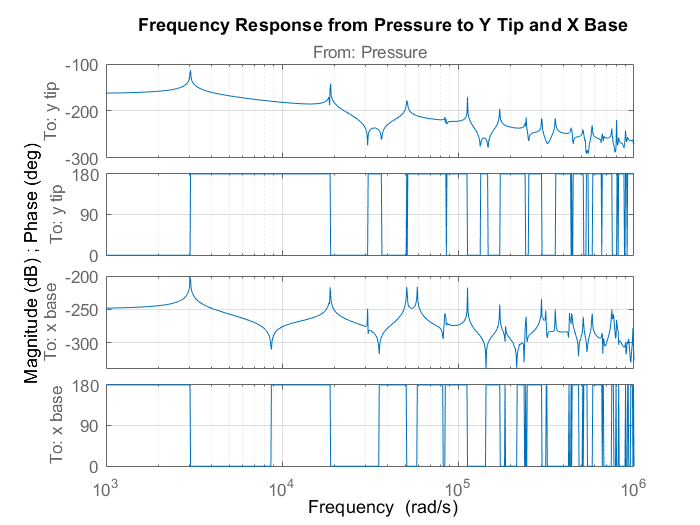
Use bode to compute the frequency response of this model.

w = logspace(3,6,1000); 
figure
bode(sys,w) 

Starting parallel pool (parpool) using the 'Processes' profile ...
04-Mar-2024 14:34:16: Job Queued. Waiting for parallel pool job with ID 1 to start ...
Connected to parallel pool with 6 workers.

grid
title("Frequency Response from Pressure to Y Tip and X Base")

The plot clearly shows the tine and the end handle vibrate at the same frequency. The first mode is at approximately 2926 rad/s and second resonance is at a frequency approximately six times higher.

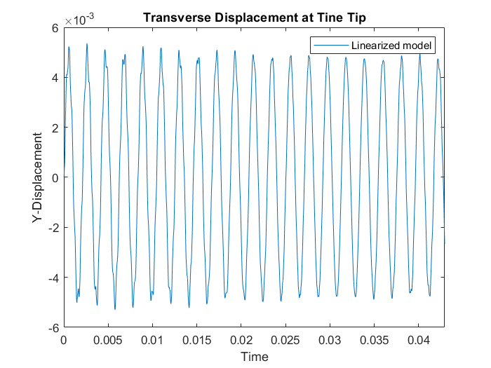
Next use lsim to obtain the impulse response of the linearized tuning fork model for 20 periods of the fundamental mode. To limit error due to linear interpolation of pressure between samples, use a step size of Te/10. The pressure is applied for the time interval [0 Te].

ncycle = 20;
Tf = ncycle*T;
h = Te/10;
t = 0:h:Tf;
u = zeros(size(t));    
u(t<=Te) = 5e6;
y = lsim(sys,u,t);

Plot the transverse displacement at the tine tip and axial displacement of the end handle.

figure
plot(t,y(:,1))
title("Transverse Displacement at Tine Tip")
xlim([0,Tf])
xlabel("Time")
ylabel("Y-Displacement")
legend("Linearized model")

figure
plot(t,y(:,2))
title("Axial Displacement at End of Handle")
xlim([0,Tf])
ylabel("X-Displacement")
xlabel("Time")
legend("Linearized model")