Multi-Loop PI Control of a Robotic Arm
This example shows how to use looptune to tune a multi-loop controller for a 6-DOF robotic arm manipulator.
Robotic Arm Model and Controller
This example uses the six degree-of-freedom robotic arm shown below. This arm consists of six joints labeled from base to tip: "Turntable", "Bicep", "Forearm", "Wrist", "Hand", and "Gripper". Each joint is actuated by a DC motor except for the Bicep joint which uses two DC motors in tandem.

Figure 1: Robotic arm manipulator.
The file cst_robotarm.slx contains a Simulink® model of the electrical and mechanical components of this system.
open_system("cst_robotarm")
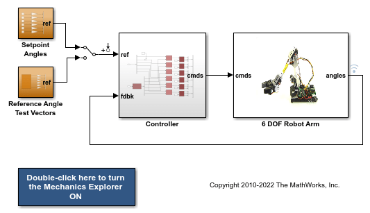
Figure 2: Simulink model of robotic arm.
The "Controller" subsystem consists of six digital PI controllers (one per joint). Each PI controller is implemented using the "2-DOF PID Controller" block from the Simulink library. For more information, see PID Tuning for Setpoint Tracking vs. Disturbance Rejection. The control sample time is Ts=0.1 (10 Hz).
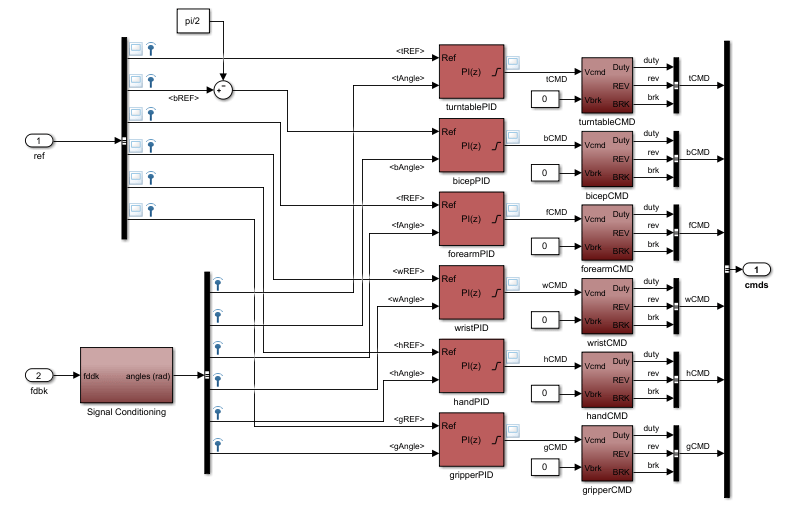
Figure 3: Controller structure.
Typically, such multi-loop controllers are tuned sequentially by tuning one PID loop at a time and cycling through the loops until the overall behavior is satisfactory. This process can be time consuming and is not guaranteed to converge to the best overall tuning. Alternatively, you can use systune or looptune to jointly tune all six PI loops subject to system-level requirements such as response time and minimum cross-coupling.
In this example, the arm must move to a particular configuration in about 1 second with smooth angular motion at each joint. The arm starts in a fully extended vertical position with all joint angles at zero except for the Bicep angle at ninety degrees. The end configuration is specified by the angular positions: Turntable = 60 deg, Bicep = 80 deg, Forearm = 60 deg, Wrist = 90 deg, Hand = 90 deg, and Gripper = 60 deg.
Press the "Play" button in the Simulink model to simulate the angular trajectories for the PI gain values specified in the model. You can first double-click the blue button to also show a 3D animation of the robotic arm. The angular responses and the 3D animation appear below. Clearly the response is too sluggish and imprecise.

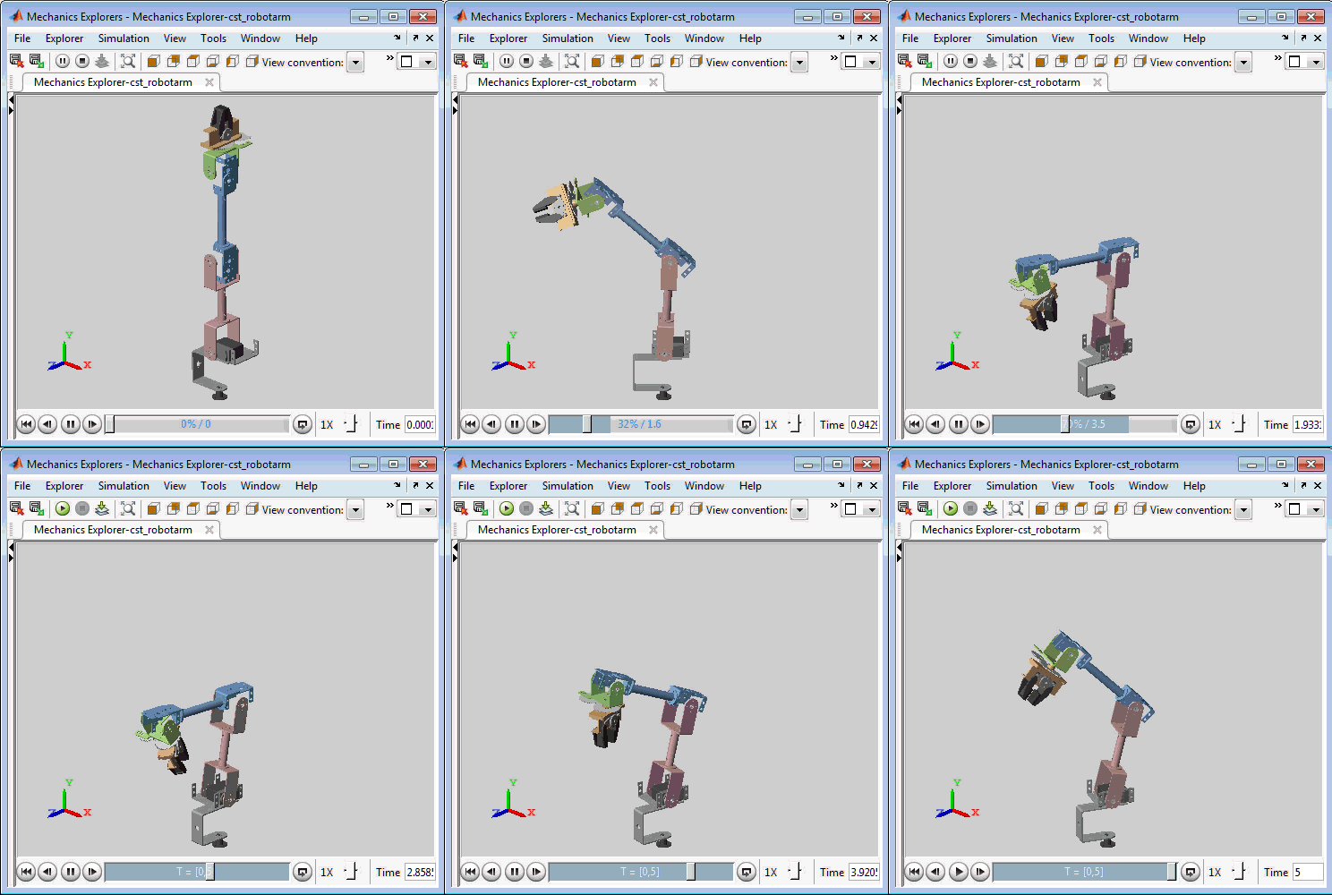
Figure 4: Untuned response.
Linearizing the Plant
The robot arm dynamics are nonlinear. To understand whether the arm can be controlled with one set of PI gains, linearize the plant at various points (snapshot times) along the trajectory of interest. Here "plant" refers to the dynamics between the control signals (outputs of PID blocks) and the measurement signals (output of "6 DOF Robot Arm" block).
SnapshotTimes = 0:1:5;

% Plant is from PID outputs to Robot Arm outputs
LinIOs = [...
   linio("cst_robotarm/Controller/turntablePID",1,"openinput"),...
   linio("cst_robotarm/Controller/bicepPID",1,"openinput"),...
   linio("cst_robotarm/Controller/forearmPID",1,"openinput"),...
   linio("cst_robotarm/Controller/wristPID",1,"openinput"),...
   linio("cst_robotarm/Controller/handPID",1,"openinput"),...
   linio("cst_robotarm/Controller/gripperPID",1,"openinput"),...
   linio("cst_robotarm/6 DOF Robot Arm",1,"output")];
LinOpt = linearizeOptions(SampleTime=0);  % seek continuous-time model
G = linearize("cst_robotarm",LinIOs,SnapshotTimes,LinOpt);

size(G)
6x1 array of state-space models.
Each model has 6 outputs, 6 inputs, and 19 states.
Plot the gap between the linearized models at t=0,1,2,3,4 seconds and the final model at t=5 seconds.
G5 = G(:,:,end);  % t=5
G5.SamplingGrid = [];
sigma(G5,G(:,:,2:5)-G5,{1e-3,1e3})
grid
title("Variation of linearized dynamics along trajectory")
legend("Linearization at t=5 s","Absolute variation",...
       Location="southwest")
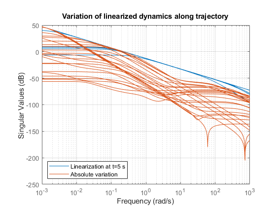
While the dynamics vary significantly at low and high frequency, the variation drops to less than 10% near 10 rad/s, which is roughly the desired control bandwidth. Small plant variations near the target gain crossover frequency suggest that we can control the arm with a single set of PI gains and need not resort to gain scheduling.
Tuning the PI Controllers with LOOPTUNE
With looptune, you can directly tune all six PI loops to achieve the desired response time with minimal loop interaction and adequate MIMO stability margins. The controller is tuned in continuous time and automatically discretized when writing the PI gains back to Simulink. Use the slTuner interface to specify which blocks must be tuned and to locate the plant/controller boundary.
% Linearize the plant at t=3s
tLinearize = 3;

% Create slTuner interface
TunedBlocks = {"turntablePID","bicepPID","forearmPID",...
               "wristPID","handPID","gripperPID"};
ST0 = slTuner("cst_robotarm",TunedBlocks,tLinearize);

% Mark outputs of PID blocks as plant inputs
addPoint(ST0,TunedBlocks)

% Mark joint angles as plant outputs
addPoint(ST0,"6 DOF Robot Arm")

% Mark reference signals
RefSignals = {...
   "ref Select/tREF",...
   "ref Select/bREF",...
   "ref Select/fREF",...
   "ref Select/wREF",...
   "ref Select/hREF",...
   "ref Select/gREF"};
addPoint(ST0,RefSignals)
In its simplest use, looptune only needs to know the target control bandwidth, which should be at least twice the reciprocal of the desired response time. Here the desired response time is 1 second so try a target bandwidth of 3 rad/s (bearing in mind that the plant dynamics vary least near 10 rad/s).
wc = 3;  % target gain crossover frequency
Controls = TunedBlocks;      % actuator commands
Measurements = "6 DOF Robot Arm";  % joint angle measurements
ST1 = looptune(ST0,Controls,Measurements,wc);
Final: Peak gain = 0.957, Iterations = 10
Achieved target gain value TargetGain=1.
A final value near or below 1 indicates that looptune achieved the requested bandwidth. Compare the responses to a step command in angular position for the initial and tuned controllers.
T0 = getIOTransfer(ST0,RefSignals,Measurements);
T1 = getIOTransfer(ST1,RefSignals,Measurements);

sp = stepplot(T0,"b--",T1,"r",4);
sp.IOGrouping = "all";
legend("Initial","Tuned",Location="southeast")
grid
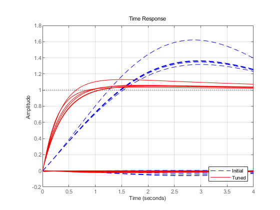
The six curves settling near y=1 represent the step responses of each joint, and the curves settling near y=0 represent the cross-coupling terms. The tuned controller is a clear improvement, but there is some overshoot and the Bicep response takes a long time to settle.
Exploiting the Second Degree of Freedom
The 2-DOF PI controllers have a feedforward and a feedback component.

Figure 5: Two degree-of-freedom PID controllers.
By default, looptune only tunes the feedback loop and does not "see" the feedforward component. This can be confirmed by verifying that the  parameters of the PI controllers remain set to their initial value
  (type
(type showTunable(ST1) to see the tuned values). To take advantage of the feedforward action and reduce overshoot, replace the bandwidth target by an explicit step tracking requirement from reference angles to joint angles.
TR = TuningGoal.StepTracking(RefSignals,Measurements,0.5);
ST2 = looptune(ST0,Controls,Measurements,TR);
Final: Peak gain = 0.766, Iterations = 13
Achieved target gain value TargetGain=1.
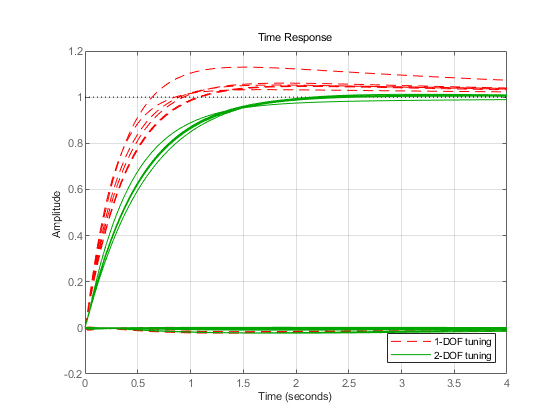
The 2-DOF tuning eliminates overshoot and improves the Bicep response.
T2 = getIOTransfer(ST2,RefSignals,Measurements);
sp = stepplot(T1,"r--",T2,"g",4);
sp.IOGrouping = "all";
legend("1-DOF tuning","2-DOF tuning",Location="southeast");
Validating the Tuned Controller
The tuned linear responses look satisfactory so write the tuned values of the PI gains back to the Simulink blocks and simulate the overall maneuver. The simulation results appear in Figure 6.
writeBlockValue(ST2)
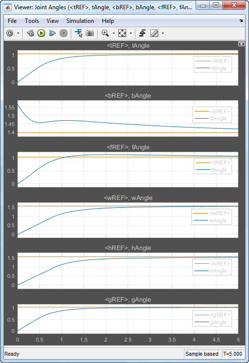
Figure 6: Tuned angular responses.
The nonlinear response of the Bicep joint noticeably undershoots. Further investigation suggests two possible culprits. First, the PI controllers are too aggressive and saturate the motors (the input voltage is limited to ± 5 V).

Figure 7: Input voltage to DC motors (control signal).
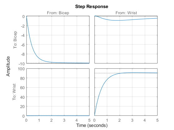
Second, cross-coupling effects between the Wrist and Bicep, when brought to scale, have a significant and lasting impact on the Bicep response. To see this, plot the step response of these three joints for the actual step changes occurring during the maneuver (-10 deg for the Bicep joint and 90 degrees for the Wrist joint).
H2 = T2([2 4],[2 4]) * diag([-10 90]);  % scale by step amplitude
H2.u = ["Bicep","Wrist"];
H2.y = ["Bicep","Wrist"];
step(H2,5)
grid
Refining the Design
To improve the Bicep response for this specific arm maneuver, we must keep the cross-couplings effects small relative to the final angular displacements in each joint. To do this, scale the cross-coupling terms in the step tracking requirement by the reference angle amplitudes.
JointDisp = [60 10 60 90 90 60];  % commanded angular displacements, in degrees
TR.InputScaling = JointDisp;
To reduce saturation of the actuators, limit the gain from reference signals to control signals.
UR = TuningGoal.Gain(RefSignals,Controls,6);
Retune the controller with these refined tuning goals.
ST3 = looptune(ST0,Controls,Measurements,TR,UR);
Final: Peak gain = 1.14, Iterations = 200
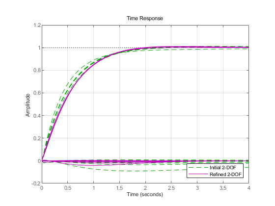
Compare the scaled responses with the previous design. Notice the significant reduction of the coupling between Wrist and Bicep motion, both in peak value and total energy.
T2s = diag(1./JointDisp) * T2 * diag(JointDisp);
T3s = diag(1./JointDisp) * getIOTransfer(ST3,RefSignals,Measurements) * diag(JointDisp);
sp = stepplot(T2s,"g--",T3s,"m",4);
sp.IOGrouping = "all";
legend("Initial 2-DOF","Refined 2-DOF",Location="southeast");
Push the retuned values to Simulink for further validation.
writeBlockValue(ST3)
The simulation results appear in Figure 8. The Bicep response is now on par with the other joints in terms of settling time and smooth transient, and there is less actuator saturation than in the previous design.

Figure 8: Angular positions and control signals with refined controller.
The 3D animation confirms that the arm now moves quickly and precisely to the desired configuration.
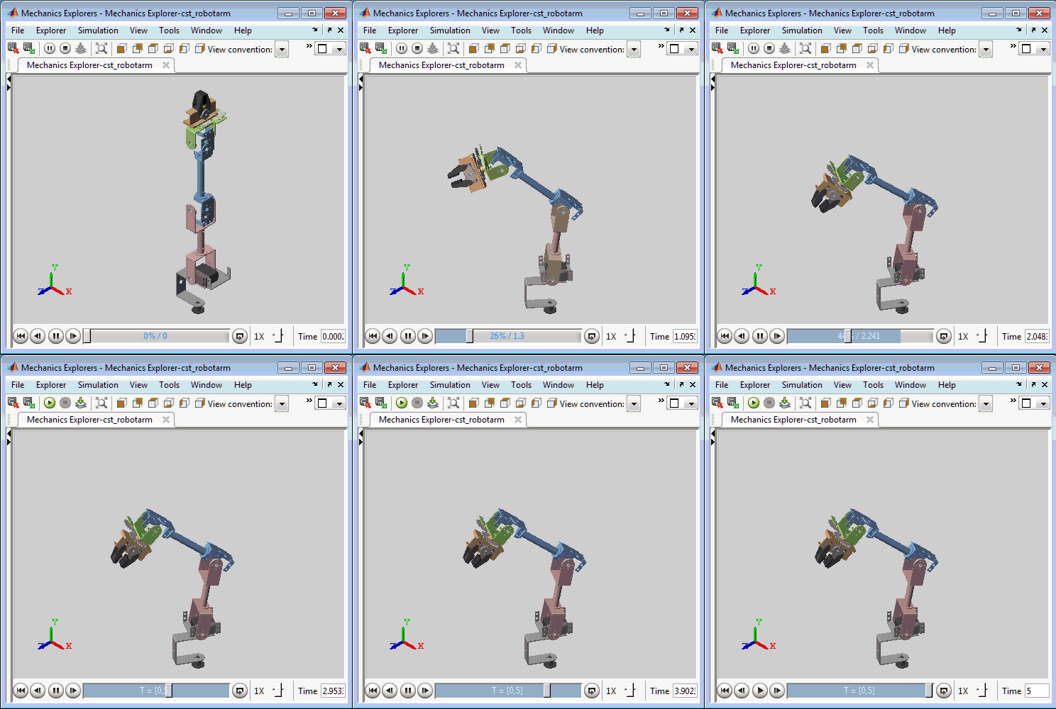
Figure 9: Fine-tuned response.
See Also
systune | TuningGoal.Tracking | TuningGoal.MinLoopGain | TuningGoal.MaxLoopGain