Tune PID Controller from Measured Plant Data in Live Editor
This example shows how to use Live Editor tasks to tune a PID controller for a plant, starting from the measured plant response to a known input signal. In this example, you use the Estimate State-Space Model task to generate code for estimating a parametric plant model. Then, you use the Convert Model Rate task to discretize the continuous-time identified model. Finally, you use the Tune PID Controller task to design a PID controller to achieve a closed-loop response that meets your design requirements. (Using Estimate State-Space Model requires a System Identification Toolbox™ license.)
Live Editor tasks let you interactively iterate on parameters and settings while observing their effects on the result of your computation. The tasks then automatically generate MATLAB® code that achieves the displayed results. To experiment with the Live Editor tasks in this script, open this example. For more information about Live Editor Tasks generally, see Add Interactive Tasks to a Live Script.
Load Plant Data
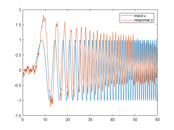
Load the measured input-output data. In this example, the data consists of the response of an engine to a chirp input. The input u is a vector containing the input signal sampled every 0.04 seconds. The output vector y contains the corresponding measured response.
load IdentPlantPIDExample u y
t = 0.04*(0:length(u)-1);
plot(t,u,t,y)
legend('input u','response y')
Estimate State-Space Model
To estimate a state-space model from this data, use the Estimate State-Space Model (System Identification Toolbox) Live Editor task. You can insert a task into your script using the Task menu in the Live Editor. In this script, Estimate State-Space Model is already inserted. Open the example to experiment with the task.
To perform the estimation, in the task, specify the input and output signals you loaded, u and y, and the sample time, 0.04 seconds. (For this example, you do not have validation data.) You also need to specify a plant order. Typically, you can guess the plant order based upon your knowledge of your system. In general, you want to use the lowest plant order that gives a reasonably good estimation fit. In the Estimate State-Space Model task, experiment with different plant order values and observe the fit result, displayed in the output plot. For details about the available options and parameters, see the Estimate State-Space Model (System Identification Toolbox) task reference page.
After you set parameters in the task, the task generates code for performing the estimation and creating a plot. To see the generated code, click ![]() Show code at the bottom of the task. When you are ready, click
Show code at the bottom of the task. When you are ready, click ![]() to run the code.
to run the code.
% Create object for time series data
estimationData = iddata(y,u,0.04);

% Estimate state-space model
sys_id = ssest(estimationData,4);

% Display results
compare(estimationData,sys_id);
clear estimationData;
title('Fit to estimation data');
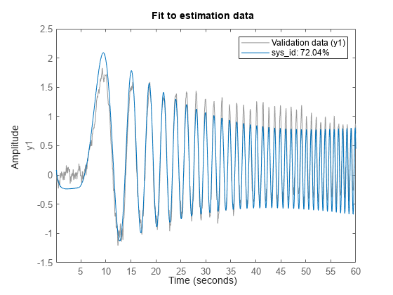
For this example, at plant order 4, the estimation fit is about 72%. Try increasing the plant order to see that doing so does not improve the fit much. Therefore, use the fourth-order plant. The code produces an identified state-space model with the variable name that you type into the summary line of the Estimate State-Space Model task. For this example, use sys_id. After you finish experimenting with the task, the identified state-space model sys_id is in the MATLAB workspace, and you can use it for additional design and analysis in the same way you use any other LTI model object. For instance, examine the frequency response of the identified state-space model sys_id.
bode(sys_id)
grid on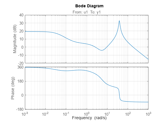
Discretize Model
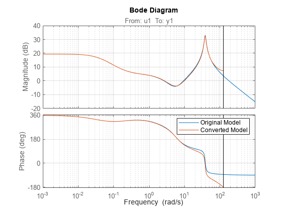
Suppose that you want to discretize this model before you design a PID controller for it. To do so, use the Convert Model Rate task. In the task, select the identified model sys_id. Specify a sample time fast enough to accommodate the resonance in the identified model response, such as 0.025 s. You can also choose a different conversion method to better match the frequency response in the vicinity of the resonance. For instance, try setting Method to Bilinear (Tustin) approximation with a prewarp frequency of 38.4 rad/s, the location of the peak response. As you experiment with settings in the task, compare the original and converted models in a Bode plot to make sure you are satisfied with the match. (For more information about the parameters and options, see the Convert Model Rate task reference page.)
Convert Model Rate generates code that produces the discretized model with the variable name that you type into the summary line of the task. For this example, use sys_d.
% Convert model from continuous to discrete time
sys_d = c2d(sys_id,0.025);

% Visualize the results
bodeplot(sys_id,sys_d);
legend('Original Model','Converted Model');
grid on;
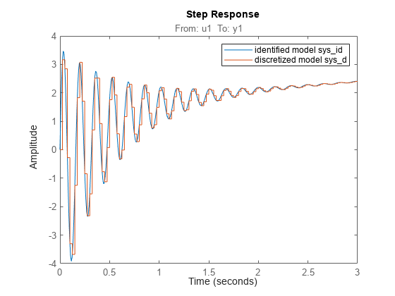
To confirm that the discretized model captures the transient response due to the resonance, compare the first few seconds of the step responses of the original identified model sys_id and the discretized model sys_d.
step(sys_id,sys_d,3)
legend('identified model sys_id','discretized model sys_d')
Tune Controller for Discretized Plant Model
Finally, use the Tune PID Controller task to generate code for tuning a PI or PID controller for the discretized plant sys_d. The task designs a PID controller for a specified plant assuming the standard unit-feedback control configuration of the following diagram.
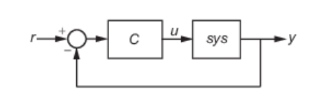
In the task, select sys_d as the plant and experiment with settings such as controller type and response time. As you change settings, select output plots on which to observe the closed-loop response generated by the task. Check System response characteristics to generate a numerical display of closed-loop step-response characteristics such as rise time and overshoot.
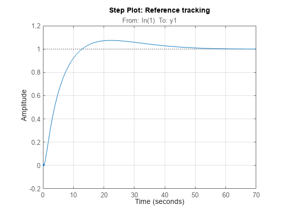
% Convert Response Time to Bandwidth
% Bandwidth is equivalent to 2 divided by the Response Time
wc = 2/11;

% PID tuning algorithm for linear plant model
[C,pidInfo] = pidtune(sys_d,'PIDF',wc);

% Clear Temporary Variables
clear wc

% Get desired loop response
Response = getPIDLoopResponse(C,sys_d,'closed-loop');

% Plot the result
stepplot(Response)
title('Step Plot: Reference tracking')
grid on
% Display system response characteristics
disp(stepinfo(Response))
RiseTime: 8.3250
TransientTime: 43.2750
SettlingTime: 43.3500
SettlingMin: 0.9008
SettlingMax: 1.0741
Overshoot: 7.4059
Undershoot: 0.5440
Peak: 1.0741
PeakTime: 22.3250
% Clear Temporary Variables
clear Response
For this example, suppose that you want the closed-loop system to settle within 50 seconds, and that the system can tolerate overshoot of no more than 10%. Adjust controller settings such as Controller Type and Response Time to achieve that target. For more information about the available parameters and options, see the Tune PID Controller task reference page.
Further Analysis of Design
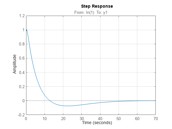
Like the other Live Editor tasks, Tune PID Controller generates code that produces a tuned controller with the variable name that you type into the summary line of the task. For this example, use C. The tuned controller C is a pid model object in the MATLAB workspace that you can use for further analysis. For example, compute the closed-loop response to a disturbance at the output of the plant sys_d, using this controller. Examine the response and its characteristics.
CLdist = getPIDLoopResponse(C,sys_d,"output-disturbance");
step(CLdist)
grid on
You can use the models sys_id, sys_d, and C for any other control design or analysis tasks.
See Also
Live Editor Tasks
- Estimate State-Space Model (System Identification Toolbox) | Convert Model Rate | Tune PID Controller