评估曲线拟合
此示例说明如何使用曲线拟合。
加载数据并拟合多项式曲线
load census
curvefit = fit(cdate,pop,'poly3','normalize','on')
curvefit =
     Linear model Poly3:
     curvefit(x) = p1*x^3 + p2*x^2 + p3*x + p4
       where x is normalized by mean 1890 and std 62.05
     Coefficients (with 95% confidence bounds):
       p1 =       0.921  (-0.9743, 2.816)
       p2 =       25.18  (23.57, 26.79)
       p3 =       73.86  (70.33, 77.39)
       p4 =       61.74  (59.69, 63.8)
输出显示拟合的模型方程、拟合的系数以及拟合系数的置信边界。
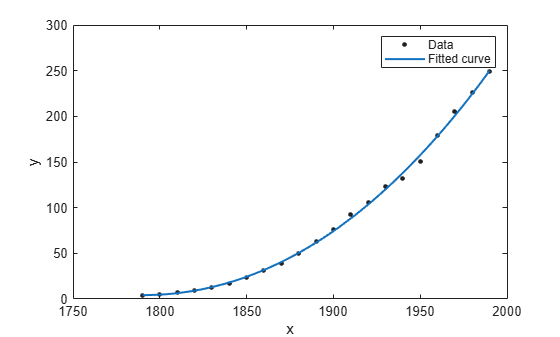
绘制拟合、数据、残差和预测边界
plot(curvefit,cdate,pop)
绘制残差拟合图。
plot(curvefit,cdate,pop,'Residuals')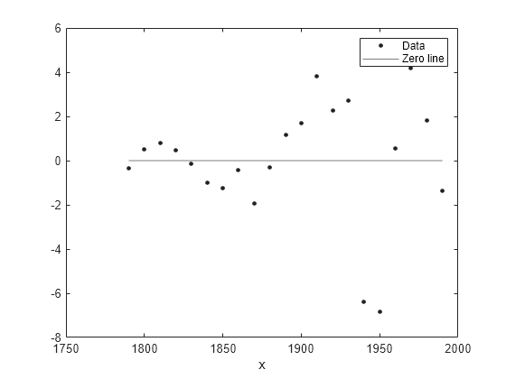
绘制拟合的预测边界。
plot(curvefit,cdate,pop,'predfunc')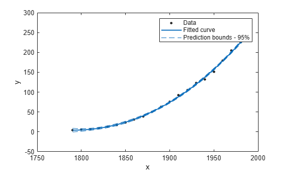
评估指定点处的拟合
使用以下格式通过指定 x 的一个值来计算特定点处的拟合:y = fittedmodel(x)。
curvefit(1991)
ans =
252.6690
评估多个点处的拟合值
计算模型在值向量处的值,将值外插到 2050 年。
xi = (2000:10:2050).';
curvefit(xi)
ans = 6×1

  276.9632
  305.4420
  335.5066
  367.1802
  400.4859
  435.4468
获取这些值的预测边界。
ci = predint(curvefit,xi)
ci = 6×2

  267.8589  286.0674
  294.3070  316.5770
  321.5924  349.4208
  349.7275  384.6329
  378.7255  422.2462
  408.5919  462.3017
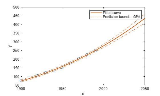
基于经外插后的拟合范围绘制拟合和预测区间图。默认情况下,系统会基于数据范围拟合图。要查看拟合的外插值,请在绘制拟合图之前将坐标区的 x 上限设置为 2050。要绘制预测区间图,请使用 predobs 或 predfun 作为绘图类型。
plot(cdate,pop,'o')
xlim([1900,2050])
hold on
plot(curvefit,'predobs')
hold off
获取模型方程
输入拟合名称以显示模型方程、拟合系数和拟合系数的置信边界。
curvefit
curvefit =
     Linear model Poly3:
     curvefit(x) = p1*x^3 + p2*x^2 + p3*x + p4
       where x is normalized by mean 1890 and std 62.05
     Coefficients (with 95% confidence bounds):
       p1 =       0.921  (-0.9743, 2.816)
       p2 =       25.18  (23.57, 26.79)
       p3 =       73.86  (70.33, 77.39)
       p4 =       61.74  (59.69, 63.8)
要仅获得模型方程,请使用 formula。
formula(curvefit)
ans =
'p1*x^3 + p2*x^2 + p3*x + p4'
获取系数名称和值
通过名称指定一个系数。
p1 = curvefit.p1
p1 =
0.9210
p2 = curvefit.p2
p2 =
25.1834
获取所有系数名称。查看拟合方程(例如 f(x) = p1*x^3+...)以查看每个系数的模型项。
coeffnames(curvefit)
ans = 4×1 cell
    {'p1'}
    {'p2'}
    {'p3'}
    {'p4'}
获取所有系数值。
coeffvalues(curvefit)
ans = 1×4

    0.9210   25.1834   73.8598   61.7444
获得系数的置信边界
使用系数的置信边界来帮助您评估和比较拟合情况。系数的置信边界确定其准确性。相距很远的边界表示存在不确定性。如果线性系数的置信边界跨越了零点,这意味着您无法确定这些系数是否与零有差异。如果一些模型项的系数为零,则它们对拟合没有影响。
confint(curvefit)
ans = 2×4

   -0.9743   23.5736   70.3308   59.6907
    2.8163   26.7931   77.3888   63.7981
检查拟合优度统计量
要在命令行中获得拟合优度统计量,您可以采用以下任一方法:
打开曲线拟合器。在曲线拟合器选项卡的导出部分中,点击导出并选择导出到工作区,以将您的拟合和拟合优度导出到工作区。
使用
fit函数指定gof输出参量。
通过指定 gof 和输出参量重新创建拟合,以获得拟合优度统计量和拟合算法信息。
[curvefit,gof,output] = fit(cdate,pop,'poly3','normalize','on')
curvefit =
     Linear model Poly3:
     curvefit(x) = p1*x^3 + p2*x^2 + p3*x + p4
       where x is normalized by mean 1890 and std 62.05
     Coefficients (with 95% confidence bounds):
       p1 =       0.921  (-0.9743, 2.816)
       p2 =       25.18  (23.57, 26.79)
       p3 =       73.86  (70.33, 77.39)
       p4 =       61.74  (59.69, 63.8)
gof = struct with fields:
           sse: 149.7687
       rsquare: 0.9988
           dfe: 17
    adjrsquare: 0.9986
          rmse: 2.9682
output = struct with fields:
        numobs: 21
      numparam: 4
     residuals: [21×1 double]
      Jacobian: [21×4 double]
      exitflag: 1
     algorithm: 'QR factorization and solve'
    iterations: 1
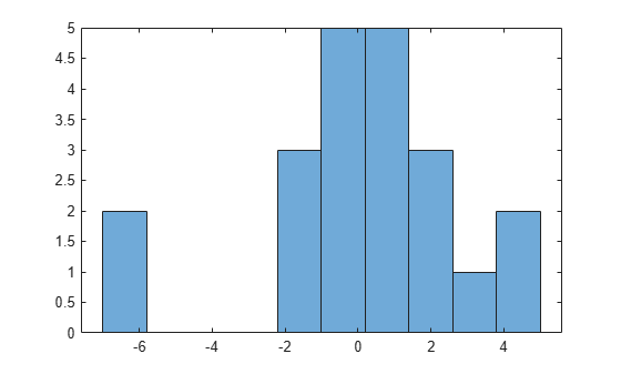
绘制残差直方图,寻找大致正态的分布。
histogram(output.residuals,10);
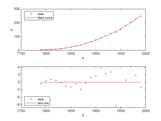
绘制拟合、数据和残差的图
figure;
plot(curvefit,cdate,pop,'fit','residuals');
legend Location SouthWest;
查找方法
列出您可以用于拟合的每种方法。
methods(curvefit)
Methods for class cfit:

argnames       category       cfit           coeffnames     coeffvalues    confint        dependnames    differentiate  feval          fitoptions     formula        indepnames     integrate      islinear       numargs        numcoeffs      plot           predint        probnames      probvalues     setoptions     type
有关如何使用拟合方法的详细信息,请参阅 cfit。