Surface Fitting to Franke Data
The Curve Fitter app provides some example data generated from Franke's bivariate test function. This data is suitable for trying various fit settings in the Curve Fitter app. Use the data to create, compare, and export surface fits.
At the MATLAB® command line, load the
frankedata set. The variablesx,y, andzappear in the workspace.load frankeThe example data is generated from Franke's bivariate test function, with added noise and scaling, to create suitable data for trying various fit settings in the Curve Fitter app. For details on the Franke function, see [1].
Divide the data into fitting and validation data.
xv = x(200:293);
yv = y(200:293);
zv = z(200:293);
x = x(1:199);
y = y(1:199);
z = z(1:199);
Fit a surface using the example data.
Open the Curve Fitter app.
Alternatively, on the Apps tab, in the Math, Statistics and Optimization group, click Curve Fitter.curveFitter
In the Curve Fitter app, select the data variables. On the Curve Fitter tab, in the Data section, click Select Data. In the Select Fitting Data dialog box, specify
xas the X data variable,yas the Y data variable, andzas the Z data variable.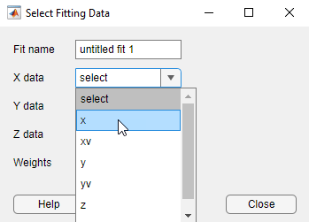
Alternatively, you can specify the data variables when you use
curveFitterto open the Curve Fitter app and create a default fit (curveFitter(x,y,z)).
The Curve Fitter app plots the data points as you select variables. When you select
x,y, andz, the app automatically creates a default surface fit. The default fit is an interpolating surface that passes through the data points.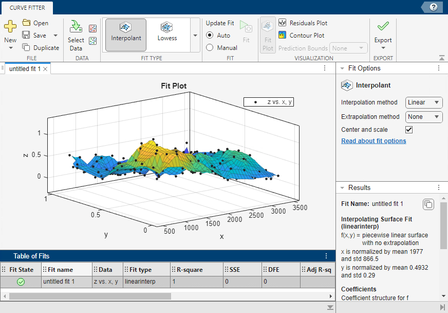
Try a Lowess fit type. On the Curve Fitter tab, in the Fit Type section, click the arrow to open the gallery. Click Lowess in the Smoothing group.
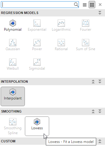
The Curve Fitter app creates a local smoothing regression fit.
Try altering the fit settings. In the Fit Options pane, change the Span (%) value to
10.By reducing the span from the default to 10% of the total number of data points, you produce a surface that follows the data more closely. The span defines the neighboring data points the app uses to determine each smoothed value.
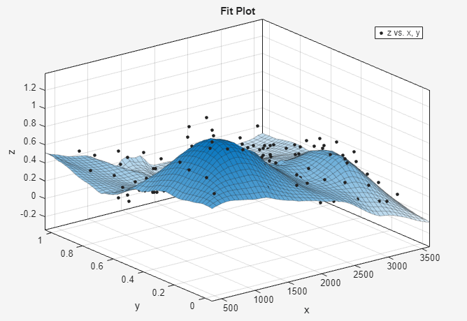
In the Table of Fits pane, change the Fit name to
Smoothing regression.Use the validation data to check that your surface is a good model. In other words, compare the surface against data not used for fitting.
On the Curve Fitter tab, in the Data section, click Validation Data. In the Select Validation Data dialog box, select the validation variables in the drop-down lists for X data, Y data, and Z data:
xv,yv, andzv.Review your selected validation data in the plots and the validation statistics (SSE and RMSE) in the Results and Table of Fits panes.
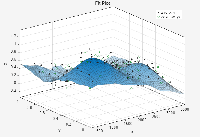
Create another fit by making a copy of the current surface fit. On the Curve Fitter tab, in the File section, click Duplicate. Alternatively, right-click the fit in the Table of Fits pane, and then select Duplicate "Smoothing regression".
The app creates a new fit figure with the same fit settings, data, and validation data. It also adds a new row to the table of fits at the bottom.
Change the fit type and name of the new fit. On the Curve Fitter tab, in the Fit Type section, click the arrow to open the gallery. Click Polynomial in the Regression Models group.
In the Table of Fits pane, change the Fit name to
Polynomial.In the Fit Options pane, change the X Degree and Y Degree values to
3, to fit a cubic polynomial in both dimensions.Look at the scales on the x and y axes, and read the warning message in the Results pane.
Equation is badly conditioned. Remove repeated data points or try centering
            and scaling.
In the Fit Options pane, select the Center and scale check box to normalize and correct for the large difference in scales in x and y.

Normalizing the surface fit removes the warning message from the Results pane.
Look at the Results pane. You can view the:
Model equation
Values of the estimated coefficients
Goodness-of-fit statistics
Goodness of validation statistics
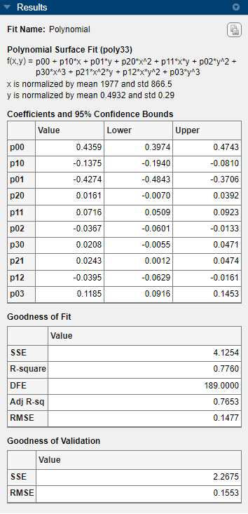
To export this fit information to the workspace, click Export and select Export to Workspace in the Export section of the Curve Fitter tab. Executing this command also exports other information such as the number of observations and parameters, residuals, and the fitted model.
You can treat the fitted model as a function to make predictions or evaluate the surface at values of X and Y. For details see Exporting a Fit to the Workspace.
Display the residuals plot to check the distribution of points relative to the surface. On the Curve Fitter tab, in the Visualization section, click Residuals Plot.

Right-click the residuals plot to select Go to X-Z view. The X-Z view is not required, but the view makes it easier to see to remove outliers.
To remove outliers, click the Exclude outliers button
 in the axes toolbar.
When you move the mouse cursor to the plot, it changes to a cross-hair to show you are in outlier selection mode.
Click a point that you want to exclude in the surface plot or residuals plot. Alternatively, click and drag to define a rectangle and remove all enclosed points.
The plots display removed points as red crosses.

If you have Auto selected in the Fit section of the Curve Fitter tab, the app refits the surface without the removed point. If you have Manual selected instead, you can click Fit to refit the surface.
To return to rotation mode in the plots, click the Exclude outliers button
 again.
Compare your fits side-by-side. Click the Document Actions button located to the far right of the fit figure tabs. Select the
Tile Alloption and specify a 1-by-2 layout.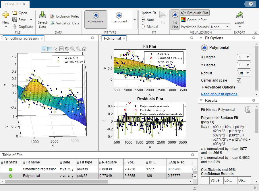
Review the information in the Table of Fits pane. Compare the goodness-of-fit statistics for all fits in your session to determine which is best.
To save your interactive surface fitting session, click Save in the File section of the Curve Fitter tab. You can save and reopen sessions to access multiple fits. The session file contains all the fits and variables in your session.
After interactively creating and comparing fits, you can generate MATLAB code for each fit in your Curve Fitter app session. On the Curve Fitter tab, in the Export section, click Export and select Generate Code.
The Curve Fitter app generates code from your session and displays the file in the MATLAB Editor. The file includes the currently selected fit and its opened plots in your session.
Save the file with the default name
createFit.m.You can recreate your fit and its plots by calling the file from the command line (with your original data or new data as input arguments). In this case, your original variables still appear in the workspace.
Highlight and evaluate the first line of the file (excluding the word
function). Either right-click and select Evaluate Selection in Command Window, press F9, or copy and paste the following code to the command line.[fitresult,gof] = createFit(x,y,z,xv,yv,zv)
The function creates a figure window for the fit you selected in your session. Observe that the polynomial fit figure shows both the surface and residuals plots that you created interactively in the Curve Fitter app.
If you want, you can use the generated code as a starting point to change the surface fits and plots to fit your needs. For a list of methods you can use, see
sfit.
References
[1] Franke, Richard. “Scattered Data Interpolation: Tests of Some Methods.” Mathematics of Computation 38, no. 157 (January 1, 1982): 181–200. https://doi.org/10.1090/S0025-5718-1982-0637296-4.