Run Sequence-to-Sequence Classification Networks with Projected Layers on FPGA

Since R2024a

This example uses:

This example shows how to create, compile, and deploy a network, that contains a projected gated recurrent unit (GRU) layer and a projected fully connected (FC) layer by using Deep Learning HDL Toolbox™. The network in this example is trained on accelerometer data from human movement. A projected layer is a type of deep learning layer that enables compression by reducing the number of stored learnable parameters. For more information about how a projected layer works, see Compress Neural Network Using Projection. Use the deployed network to classify human activity based on sequence input data. Use MATLAB® to retrieve the prediction results from the target device.

This example uses sensor data obtained from a smartphone worn on the body and deploys a GRU network trained to recognize the activity of the wearer based on time series data that represents accelerometer readings in three different directions. The training data contains time series data for seven people. Each sequence has three features and varies in length.

Prerequisites

Intel Arria® 10 SoC development board
Deep Learning HDL Toolbox™ Support Package for Intel® FPGA and SoC
Deep Learning Toolbox™
Deep Learning HDL Toolbox™
Deep Learning Toolbox Model Quantization Library

Load Pretrained Network and Data

Load the HumanActivityDataAndNetwork.mat file. This file contains the pretrained human body movement classification network and the human activity data. The data is randomly divided into training data and testing data

load HumanActivityDataAndNetwork.mat

View the network layers. The network is a GRU network with a single GRU layer that has 400 hidden units and an FC layer with five outputs that represent five activity categories.

net.Layers

ans = 
  4×1 Layer array with layers:

     1   'sequenceinput'   Sequence Input    Sequence input with 3 dimensions
     2   'gru'             GRU               GRU with 400 hidden units
     3   'fc'              Fully Connected   5 fully connected layer
     4   'softmax'         Softmax           softmax

View the category names.

categories(YTestData)

ans = 5×1 cell
    {'Dancing' }
    {'Running' }
    {'Sitting' }
    {'Standing'}
    {'Walking' }

This example tests several versions of the original network. For comparison, create a copy of the original network using a GRU layer.

netGRU = net;

Test the Pretrained Network

Calculate the classification accuracy of the original GRU network using the testing data.

netPred = netGRU.predict(XTestData');

Convert the network output to categorical labels that correspond to the activity at each time step by using the onehotdecode function.

Cats = categories(YTestData);
GRUPred = onehotdecode(netPred', Cats, 1);

Calculate the prediction accuracy of the original GRU network.

accuracyGRU = nnz(GRUPred == YTestData) / numel(YTestData)

accuracyGRU = 0.9197

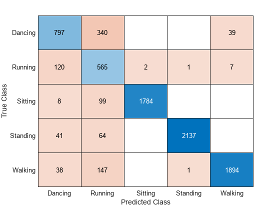
Display the prediction results in a confusion chart.

figure
confusionchart(GRUPred, YTestData);

Figure contains an object of type ConfusionMatrixChart.

Project Network

Compress the network using projection and reduce 95% of the network learnables such as weights, biases, and so on.

reductionGoal = 0.95;
data = dlarray(XTrainData, 'CBT');
netProj = compressNetworkUsingProjection(netGRU, data, LearnablesReductionGoal=reductionGoal)

Compressed network has 95.1% fewer learnable parameters.
Projection compressed 2 layers: "gru","fc"

netProj = 
  dlnetwork with properties:

         Layers: [4×1 nnet.cnn.layer.Layer]
    Connections: [3×2 table]
     Learnables: [9×3 table]
          State: [1×3 table]
     InputNames: {'sequenceinput'}
    OutputNames: {'softmax'}
    Initialized: 1

  View summary with summary.

Unpack the compressed network. You must unpack projected layers before deploying them to an FPGA.

netProj = unpackProjectedLayers(netProj);

View the compressed network.

netProj.Layers

ans = 
  5×1 Layer array with layers:

     1   'sequenceinput'   Sequence Input    Sequence input with 3 dimensions
     2   'gru'             Projected GRU     Projected GRU layer with 400 hidden units, an output projector size of 12, and an input projector size of 2
     3   'fc_proj_in'      Fully Connected   2 fully connected layer
     4   'fc_proj_out'     Fully Connected   5 fully connected layer
     5   'softmax'         Softmax           softmax

Test Projected Network

Calculate the classification accuracy of the projected network by using the testing data.

netPred = netProj.predict(XTestData');

Convert the network output to categorical labels that correspond to the activity at each time step by using the onehotdecode function.

ProjPred = onehotdecode(netPred', Cats, 1);

Calculate the prediction accuracy of the compressed network using projection. The prediction accuracy decreased because of the compression. You must fine-tune the network to improve the accuracy.

accuracyProj = nnz(ProjPred == YTestData) / numel(YTestData)

accuracyProj = 0.3859

Fine-Tune Compressed Network

Compressing a network using projection typically reduces the network accuracy. To improve the accuracy, retrain the compressed network. Retraining the network takes several hours. To retrain the network, enter:

maxEpochNum = 1000;
options = trainingOptions('adam', ...
    'MaxEpochs',maxEpochNum, ...
    'GradientThreshold',2, ...
    'Verbose',0, ...
    'Plots','training-progress');
netFT = trainnet(XTrainData',YTrainData',netProj,"crossentropy",options);

Alternatively, the HumanActivityDataAndNetwork.mat file contains the variable netFT, which contains the retrained network.

Test Fine-Tuned Network

Calculate the classification accuracy of the fine-tuned network by using the testing data.

netPred = netFT.predict(XTestData');

Convert network output to categorical labels that correspond to the activity at each time step by using the onehotdecode function

FTPred = onehotdecode(netPred', Cats, 1);

Calculate the prediction accuracy of the fine-tuned GRU projected network.

accuracyFT = nnz(FTPred == YTestData) / numel(YTestData)

accuracyFT = 0.8878

Display the prediction results in a confusion chart.

figure
confusionchart(FTPred, YTestData);

Figure contains an object of type ConfusionMatrixChart.

Compare the accuracy and the number of learnables in the original GRU network and the fine-tuned network in a bar chart. To calculate the number of learnables in each network, use the numLearnables helper function.

figure
tiledlayout("flow")

nexttile
bar([accuracyGRU accuracyProj accuracyFT])
xticklabels(["Original" "Projected" "Fine-tuned"])
title("Accuracy")
ylabel("Accuracy")

nexttile
bar([numLearnables(netGRU) numLearnables(netProj) numLearnables(netFT)])
xticklabels(["Original" "Projected" "Fine-tuned"])
ylabel("Number of Learnables")
title("Number of Learnables")

Figure contains 2 axes objects. Axes object 1 with title Accuracy, ylabel Accuracy contains an object of type bar. Axes object 2 with title Number of Learnables, ylabel Number of Learnables contains an object of type bar.

Deploy Original GRU Network on FPGA

Define the target FPGA board programming interface by using the dlhdl.Target object. Specify that the interface is for a Xilinx board with an Ethernet interface.

To create the target object, enter:

hTarget = dlhdl.Target('Intel', Interface="JTAG");

Next prepare the network for deployment by creating a dlhdl.Workflow object. Specify the network and bitstream name. Ensure that the bitstream name matches the data type and FPGA board. In this example the target FPGA board is the Xilinx ZCU102 SOC board and the bitstream uses a single data type.

hW = dlhdl.Workflow(Network=netGRU, Bitstream="arria10soc_lstm_single",Target=hTarget);

Compile Network

Run the compile method of the dlhdl.Workflow object to compile the network and generate the instructions, weights, and biases for deployment. Because the total number of frames exceeds the default value of 30, set the InputFrameNumberLimit name-value argument to prevent timeouts.

hW.compile('InputFrameNumberLimit', size(XTestData, 2));

### Compiling network for Deep Learning FPGA prototyping ...
### Targeting FPGA bitstream arria10soc_lstm_single.
### An output layer called 'Output1_softmax' of type 'nnet.cnn.layer.RegressionOutputLayer' has been added to the provided network. This layer performs no operation during prediction and thus does not affect the output of the network.
### The network includes the following layers:
     1   'sequenceinput'     Sequence Input      Sequence input with 3 dimensions  (SW Layer)
     2   'gru'               GRU                 GRU with 400 hidden units         (HW Layer)
     3   'fc'                Fully Connected     5 fully connected layer           (HW Layer)
     4   'softmax'           Softmax             softmax                           (SW Layer)
     5   'Output1_softmax'   Regression Output   mean-squared-error                (SW Layer)
                                                                                 
### Notice: The layer 'sequenceinput' with type 'nnet.cnn.layer.ImageInputLayer' is implemented in software.
### Notice: The layer 'softmax' with type 'nnet.cnn.layer.SoftmaxLayer' is implemented in software.
### Notice: The layer 'Output1_softmax' with type 'nnet.cnn.layer.RegressionOutputLayer' is implemented in software.
### Compiling layer group: gru.wh ...
### Compiling layer group: gru.wh ... complete.
### Compiling layer group: gru.rh ...
### Compiling layer group: gru.rh ... complete.
### Compiling layer group: gru.w1 ...
### Compiling layer group: gru.w1 ... complete.
### Compiling layer group: gru.w2 ...
### Compiling layer group: gru.w2 ... complete.
### Compiling layer group: fc ...
### Compiling layer group: fc ... complete.

### Allocating external memory buffers:

          offset_name          offset_address     allocated_space  
    _______________________    ______________    __________________

    "InputDataOffset"           "0x00000000"     "128.0 kB"        
    "OutputResultOffset"        "0x00020000"     "508.0 kB"        
    "SchedulerDataOffset"       "0x0009f000"     "648.0 kB"        
    "SystemBufferOffset"        "0x00141000"     "20.0 kB"         
    "InstructionDataOffset"     "0x00146000"     "4.0 kB"          
    "FCWeightDataOffset"        "0x00147000"     "1.9 MB"          
    "EndOffset"                 "0x00329000"     "Total: 3236.0 kB"

### Network compilation complete.

Program Bitstream onto FGPA and Download Network Weights

To deploy the network on the Xilinx ZCU102 SoC hardware, run the deploy method of the dlhdl.Workflow object. This function uses the output of the compile function to program the FPGA board and download the network weights and biases. The deploy function programs the FPGA device and displays progress messages and the required time to deploy the network.

hW.deploy

### FPGA bitstream programming has been skipped as the same bitstream is already loaded on the target FPGA.
### Resetting network state.
### Loading weights to FC Processor.
### 50% finished, current time is 12-Dec-2023 17:16:13.
### FC Weights loaded. Current time is 12-Dec-2023 17:16:14

Run Prediction for the Testing Data

[FPGAResultOriginal, speedOriginal] = hW.predict(dlarray(XTestData, "CT"), 'Profile', 'on');

### Resetting network state.
### Finished writing input activations.
### Running a sequence of length 8084.


              Deep Learning Processor Profiler Performance Results

                   LastFrameLatency(cycles)   LastFrameLatency(seconds)       FramesNum      Total Latency     Frames/s
                         -------------             -------------              ---------        ---------       ---------
Network                      46948                  0.00031                    8084          383322247           3163.4
    gru.wh                     412                  0.00000 
    gru.rh                   13543                  0.00009 
    memSeparator_0              84                  0.00000 
    memSeparator_2             307                  0.00000 
    gru.w1                   13529                  0.00009 
    gru.w2                   13691                  0.00009 
    gru.sigmoid_1              349                  0.00000 
    gru.sigmoid_2              347                  0.00000 
    gru.multiplication_2       441                  0.00000 
    gru.multiplication_4       477                  0.00000 
    gru.multiplication_1       447                  0.00000 
    gru.addition_2             437                  0.00000 
    gru.addition_1             447                  0.00000 
    gru.tanh_1                 361                  0.00000 
    gru.multiplication_3       471                  0.00000 
    gru.addition_3             451                  0.00000 
    fc                         853                  0.00001 
    memSeparator_1             301                  0.00000 
 * The clock frequency of the DL processor is: 150MHz

Deploy Fine-tuned GRU Projected Network on FPGA

Prepare the network for deployment by creating a dlhdl.Workflow object. Specify the network and bitstream name. Ensure that the bitstream name matches the data type and FPGA board. In this example the target FPGA board is the Xilinx ZCU102 SOC board. The bitstream uses a single data type.

hW = dlhdl.Workflow(Network=netFT, Bitstream="arria10soc_lstm_single",Target=hTarget);

Compile Network

dn = hW.compile('InputFrameNumberLimit', size(XTestData, 2));

### Compiling network for Deep Learning FPGA prototyping ...
### Targeting FPGA bitstream arria10soc_lstm_single.
### An output layer called 'Output1_softmax' of type 'nnet.cnn.layer.RegressionOutputLayer' has been added to the provided network. This layer performs no operation during prediction and thus does not affect the output of the network.
### The network includes the following layers:
     1   'sequenceinput'     Sequence Input      Sequence input with 3 dimensions                                                                             (SW Layer)
     2   'gru'               Projected GRU       Projected GRU layer with 400 hidden units, an output projector size of 12, and an input projector size of 2  (HW Layer)
     3   'fc_proj_in'        Fully Connected     2 fully connected layer                                                                                      (HW Layer)
     4   'fc_proj_out'       Fully Connected     5 fully connected layer                                                                                      (HW Layer)
     5   'softmax'           Softmax             softmax                                                                                                      (SW Layer)
     6   'Output1_softmax'   Regression Output   mean-squared-error                                                                                           (SW Layer)
                                                                                                                                                            
### Notice: The layer 'sequenceinput' with type 'nnet.cnn.layer.ImageInputLayer' is implemented in software.
### Notice: The layer 'softmax' with type 'nnet.cnn.layer.SoftmaxLayer' is implemented in software.
### Notice: The layer 'Output1_softmax' with type 'nnet.cnn.layer.RegressionOutputLayer' is implemented in software.
### Compiling layer group: gru.inProj ...
### Compiling layer group: gru.inProj ... complete.
### Compiling layer group: gru.outProj ...
### Compiling layer group: gru.outProj ... complete.
### Compiling layer group: gru.wh ...
### Compiling layer group: gru.wh ... complete.
### Compiling layer group: gru.rh ...
### Compiling layer group: gru.rh ... complete.
### Compiling layer group: gru.w1 ...
### Compiling layer group: gru.w1 ... complete.
### Compiling layer group: gru.w2 ...
### Compiling layer group: gru.w2 ... complete.
### Compiling layer group: fc_proj_in>>fc_proj_out ...
### Compiling layer group: fc_proj_in>>fc_proj_out ... complete.

### Allocating external memory buffers:

          offset_name          offset_address     allocated_space  
    _______________________    ______________    __________________

    "InputDataOffset"           "0x00000000"     "128.0 kB"        
    "OutputResultOffset"        "0x00020000"     "508.0 kB"        
    "SchedulerDataOffset"       "0x0009f000"     "712.0 kB"        
    "SystemBufferOffset"        "0x00151000"     "20.0 kB"         
    "InstructionDataOffset"     "0x00156000"     "4.0 kB"          
    "FCWeightDataOffset"        "0x00157000"     "124.0 kB"        
    "EndOffset"                 "0x00176000"     "Total: 1496.0 kB"

### Network compilation complete.

Program Bitstream onto FGPA and Download Network Weights

hW.deploy

### FPGA bitstream programming has been skipped as the same bitstream is already loaded on the target FPGA.
### Resetting network state.
### Loading weights to FC Processor.
### FC Weights loaded. Current time is 12-Dec-2023 17:16:49

Run Prediction for the Testing Data

[FPGAResultFT, speedFT] = hW.predict(dlarray(XTestData, "CT"), 'Profile', 'on');

### Resetting network state.
### Finished writing input activations.
### Running a sequence of length 8084.


              Deep Learning Processor Profiler Performance Results

                   LastFrameLatency(cycles)   LastFrameLatency(seconds)       FramesNum      Total Latency     Frames/s
                         -------------             -------------              ---------        ---------       ---------
Network                       9459                  0.00006                    8084           81343693          14907.1
    gru.id                     348                  0.00000 
    gru.inProj                 170                  0.00000 
    gru.outProj                869                  0.00001 
    gru.wh                     362                  0.00000 
    gru.rh                     847                  0.00001 
    gru.w1                     846                  0.00001 
    gru.w2                     837                  0.00001 
    gru.sigmoid_1              370                  0.00000 
    gru.sigmoid_2              431                  0.00000 
    gru.multiplication_2       447                  0.00000 
    gru.multiplication_4       457                  0.00000 
    gru.multiplication_1       447                  0.00000 
    gru.addition_2             477                  0.00000 
    gru.addition_1             361                  0.00000 
    gru.tanh_1                 421                  0.00000 
    gru.multiplication_3       461                  0.00000 
    gru.addition_3             301                  0.00000 
    memSeparator_0              44                  0.00000 
    fc_proj_in                 847                  0.00001 
    fc_proj_out                115                  0.00000 
 * The clock frequency of the DL processor is: 150MHz

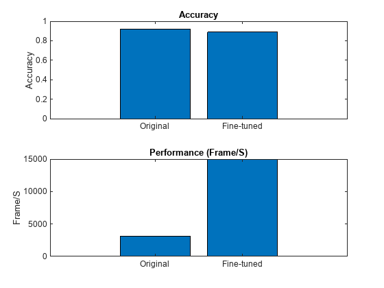
Performance Improvement From Compression

Compare the accuracy and the number of learnables in the original network and the compressed and fine-tuned network in a bar chart. To calculate the number of learnables in each network, use the numLearnables helper function.

The projected network has only 5% learnable parameters in comparison to the original GRU network, but performs 4.7 times faster when executed on Arria10soc FPGA. After the fine-tuning, the projected network has a classification accuracy similar to that of the original network.

figure
tiledlayout("flow")

nexttile
bar([accuracyGRU accuracyFT])
xticklabels(["Original" "Fine-tuned"])
title("Accuracy")
ylabel("Accuracy")

nexttile
bar([str2double(speedOriginal{1,end}), str2double(speedFT{1,end})])
xticklabels(["Original" "Fine-tuned"])
ylabel("Frame/S")
title("Performance (Frame/S)")

Figure contains 2 axes objects. Axes object 1 with title Accuracy, ylabel Accuracy contains an object of type bar. Axes object 2 with title Performance (Frame/S), ylabel Frame/S contains an object of type bar.

Supporting Functions

Number of Learnables Function

The numLearnables function returns the total number of learnables in a network.

function N = numLearnables(net)

N = 0;
for i = 1:size(net.Learnables,1)
    N = N + numel(net.Learnables.Value{i});
end

end

Run Sequence-to-Sequence Classification Networks with Projected Layers on FPGA

Prerequisites

Load Pretrained Network and Data

Test the Pretrained Network

Project Network

Test Projected Network

Fine-Tune Compressed Network

Test Fine-Tuned Network

Deploy Original GRU Network on FPGA

Compile Network

Program Bitstream onto FGPA and Download Network Weights

Run Prediction for the Testing Data

Deploy Fine-tuned GRU Projected Network on FPGA

Compile Network

Program Bitstream onto FGPA and Download Network Weights

Run Prediction for the Testing Data

Performance Improvement From Compression

Supporting Functions

Number of Learnables Function

See Also

Related Topics

Run Sequence-to-Sequence Classification Networks with Projected Layers on FPGA

Prerequisites

Load Pretrained Network and Data

Test the Pretrained Network

Project Network

Test Projected Network

Fine-Tune Compressed Network

Test Fine-Tuned Network

Deploy Original GRU Network on FPGA

Compile Network

Program Bitstream onto FGPA and Download Network Weights

Run Prediction for the Testing Data

Deploy Fine-tuned GRU Projected Network on FPGA

Compile Network

Program Bitstream onto FGPA and Download Network Weights

Run Prediction for the Testing Data

Performance Improvement From Compression

Supporting Functions

Number of Learnables Function

See Also

Related Topics

WeChat