Build Transformer Network for Time Series Regression

Load Data

Load and display the engine data timetable.

load SIEngineData.mat IOData
stackedplot(IOData)
title("SI Engine Signals")

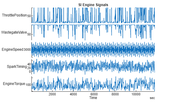
The raw data contains over one hundred thousand observations of engine torque (the response) as a function of these predictor variables, measured at 10 Hz:

Preprocess Data

To improve the performance of the transformer networks, divide the engine torque data into a cell array with windows of 40 seconds each. This division lets you build networks with fewer learnable parameters (for example, in the position encoding), reduces memory requirements for the transformer, and speeds up training. This division also moves the data from the time dimension to the batch dimension. In the batch dimension, the data is processed in parallel. As a result, the network sees more data at any given time during training, further speeding up training. The Time Series Modeler app can split a single time series into windows but in this example, the data has multiple time series, so you must manually split the data.

To speed up model training, downsample the time series from 10 Hz to 2 Hz. This also ensures that each timetable is regularly sampled, which is necessary when using Time Series Modeler.

windowLength = 400;
numWindows = floor(size(IOData,1)/windowLength);
reducedSampleRate = 2;
for i=1:numWindows
    windowIdx = 1 + (i-1)*windowLength:i*windowLength;
    data = IOData(windowIdx,:);
    windowedData{i} = retime(data,"regular","linear",SampleRate=reducedSampleRate);
end

Train Transformer Network in Time Series Modeler App

Import Data

Open the Time Series Modeler app.

timeSeriesModeler

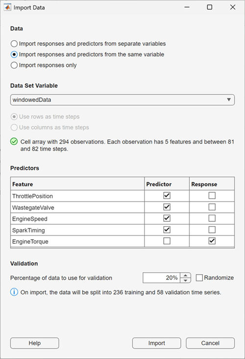
To import the predictors and responses into the app, click the New button on the toolstrip. The Import Data dialog box opens.

In the Import Data dialog box, select Import responses and predictors from the same variable and import the windowedData variable. Select Response for the EngineTorque feature, and verify that Predictor is selected for all other features. To use the last 20% of the time series as validation data, keep the default value of 20% in the Percentage of data to use for validation box. Click Import.

To verify that the data is correct, on the Data tab, view the Observation Preview pane. To display the predictor channels, in the Observation Preview pane, set the Type to Predictor. The app displays four predictor channels, each corresponding to one of the predictors, such as ThrottlePosition.

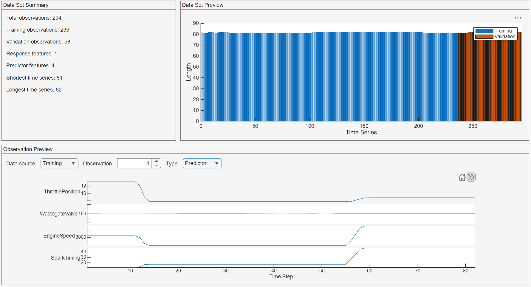
In the Data Set Summary panel, observe that the longest time series has a length of 82 time steps. This length is an important parameter for configuring the transformer network.

Build Transformer Network

This section shows you how to build a self-attention-based transformer with sinusoidal position encoding and Gaussian error linear unit (GeLU) activation layers. This transformer is based on the original transformer architecture in the "Attention is All You Need" paper [1]. To train the network faster, limit the number of learnable parameters by using an output size of 32 in fully connected layers and 32 query channels in self-attention layers.

To load a prebuilt network instead of creating the network, skip to the Load Prebuilt Network section.

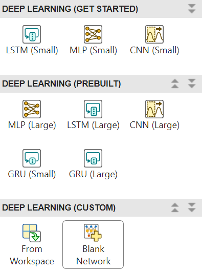
These steps show you how to create the network. Expand the Models gallery, select Blank Network.

The Customize Network dialog box opens. Keep the default settings and click Create. The Customize Network window opens.

The Customize Network window shows the sequence input layer, the output fully connected layer, and the output inverse normalization layer. The output fully connected layer has an output size of 1, which corresponds to the response you are trying to predict (the engine torque).

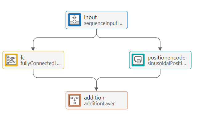
Build the rest of the transformer architecture. First, build the position encoding block:

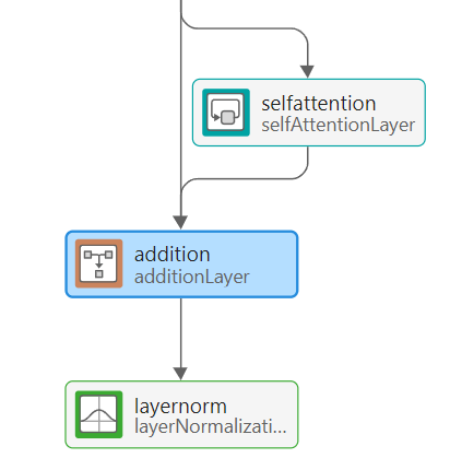
Next, build the self-attention block:

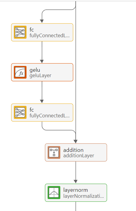
Add the fully connected block after the layer normalization layer:

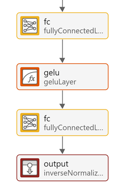
Finally, add the regression head:

Your final transformer network must look like this network.

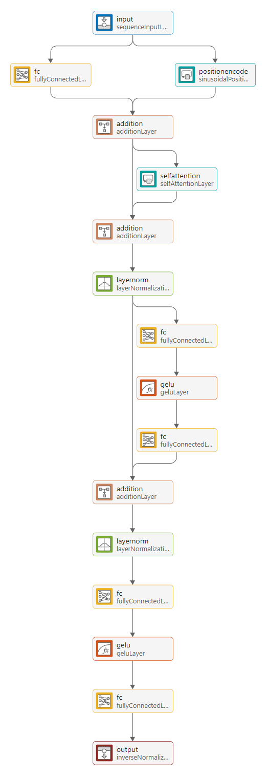
Check that all internal fully connected layers have an output size of 32, that the position encoding has an output size of 32, and that the self-attention layer has 32 query channels.

Load Prebuilt Network

Instead of building your own network, you can use the prebuilt network provided as a supporting file with this example. To use this prebuilt network, load the network and import it in the Time Series Modeler app.

load transformer_model.mat

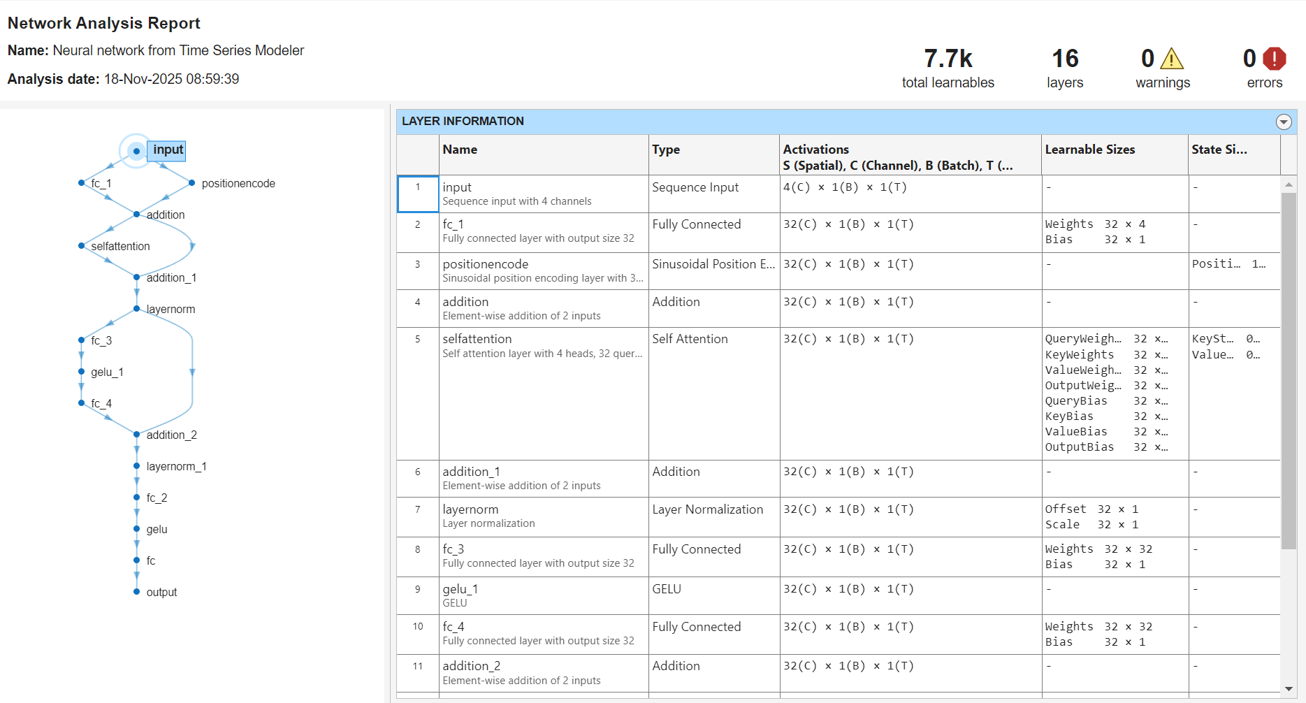
Analyze Network

To verify that you have constructed the network correctly, select Analyze. This transformer network is small and has only 7.7k learnable parameters.

To accept the changes to the network, click Accept Changes.

Train Transformer Network

In Time Series Modeler, Click Train. The network will train on your GPU if one is available. Training on a GPU takes a couple of minutes.

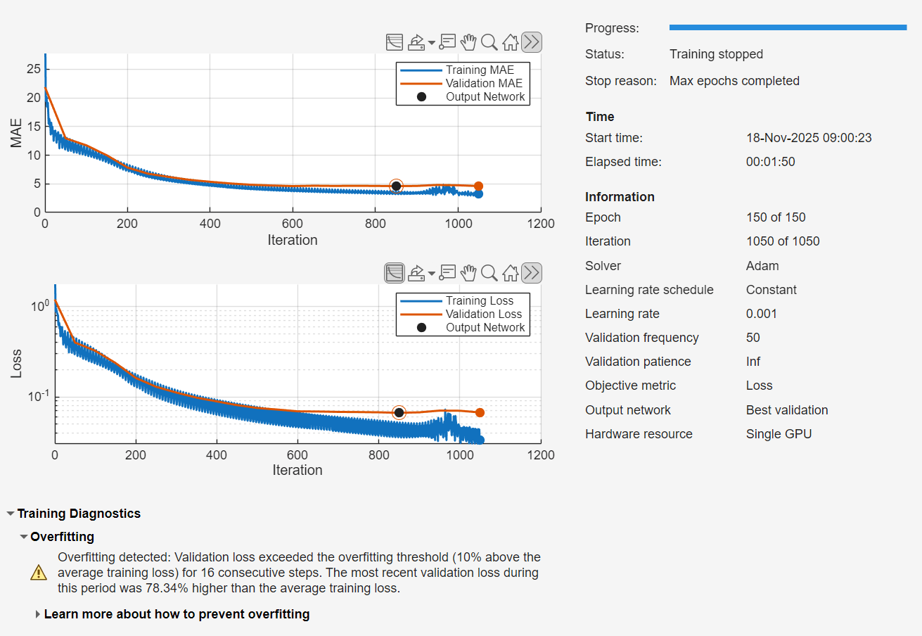
Reduce Overfitting

The transformer model overfits the training data, resulting in a high validation error. To reduce validation error and overfitting, use a causal mask for the attention layer and a dropout layer. Causal masking ensures the attention layer in the transformer network only uses past values of the time series. Dropout randomly zeros out inputs at training time and forces the network to learn features that generalize to unseen data.

To create an untrained copy of the transformer network, right-click the trained custom network in the model list on the left, and select Duplicate. Select Customize Network and make these changes to the network:

Accept the changes, and train the network.

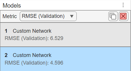
The causal mask and the dropout layer have improved the performance of the network. The transformer no longer overfits, and the validation and training loss match closely.

Small transformers, like the one used in this example, train fast on a GPU. This custom network also has a better validation root mean squared error (RMSE) compared to the default LSTM. If you have sufficient amount of data, use a transformer network as it usually outperforms simpler options such as MLP or LSTM, and is usually faster to train than an LSTM.

References

[1] Vaswani, Ashish, Noam Shazeer, Niki Parmar, Jakob Uszkoreit, Llion Jones, Aidan N. Gomez, Łukasz Kaiser, and Illia Polosukhin. "Attention is all you need." In Advances in Neural Information Processing Systems, Vol. 30. Curran Associates, Inc., 2017. https://papers.nips.cc/paper/7181-attention-is-all-you-need.