基于深度学习网络的鸡尾酒会信源分离
此示例说明如何使用深度学习网络隔离语音信号。
简介
鸡尾酒会效应指大脑专注于单个说话者而同时滤除其他声音和背景噪声的能力。人类在鸡尾酒会问题上表现很好。此示例说明如何使用深度学习网络将单个说话者从一男一女同时说话的混合语音中分离出来。
下载所需文件
在进入示例的具体步骤前,您需要下载预训练网络和 4 个音频文件。
downloadFolder = matlab.internal.examples.downloadSupportFile("audio/examples","cocktailpartyfc.zip");
dataFolder = tempdir;
dataset = fullfile(dataFolder,"CocktailPartySourceSeparation");
unzip(downloadFolder,dataset)
问题摘要
加载音频文件,其中包含以 4 kHz 采样的男性和女性语音。单独收听音频文件以供参考。
[mSpeech,Fs] = audioread(fullfile(dataset,"MaleSpeech-16-4-mono-20secs.wav"));
sound(mSpeech,Fs)
[fSpeech] = audioread(fullfile(dataset,"FemaleSpeech-16-4-mono-20secs.wav"));
sound(fSpeech,Fs)将两个语音源合并。确保信号源在混音中具有相同的功率。对混音进行缩放,使其最大振幅为 1。
mSpeech = mSpeech/norm(mSpeech);
fSpeech = fSpeech/norm(fSpeech);

ampAdj = max(abs([mSpeech;fSpeech]));
mSpeech = mSpeech/ampAdj;
fSpeech = fSpeech/ampAdj;

mix = mSpeech + fSpeech;
mix = mix./max(abs(mix));
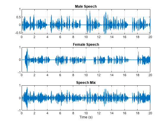
可视化原始信号和混音信号。收听混音信号。此示例说明从混合语音中提取男性和女性语音源的信源分离方案。
t = (0:numel(mix)-1)*(1/Fs);

figure
tiledlayout(3,1)

nexttile
plot(t,mSpeech)
title("Male Speech")
grid on

nexttile
plot(t,fSpeech)
title("Female Speech")
grid on

nexttile
plot(t,mix)
title("Speech Mix")
xlabel("Time (s)")
grid on
收听混合音频。
sound(mix,Fs)
时频表示
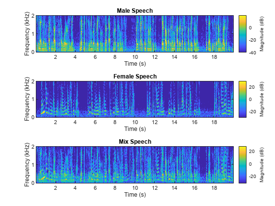
使用 stft 可视化男性语音、女性语音和混合语音信号的时频表示 (TF)。使用长度为 128、FFT 长度为 128 且重叠长度为 96 的汉宁窗。
windowLength = 128;
fftLength = 128;
overlapLength = 96;
win = hann(windowLength,"periodic");

figure
tiledlayout(3,1)

nexttile
stft(mSpeech,Fs,Window=win,OverlapLength=overlapLength,FFTLength=fftLength,FrequencyRange="onesided");
title("Male Speech")

nexttile
stft(fSpeech,Fs,Window=win,OverlapLength=overlapLength,FFTLength=fftLength,FrequencyRange="onesided");
title("Female Speech")

nexttile
stft(mix,Fs,Window=win,OverlapLength=overlapLength,FFTLength=fftLength,FrequencyRange="onesided");
title("Mix Speech")
使用理想时频掩膜的信源分离
TF 掩膜的应用已被证明是从多源声音中分离期望的音频信号的有效方法。TF 掩膜是与基础 STFT 大小相同的矩阵。该掩膜与基础 STFT 逐元素相乘以隔离期望的信源。TF 掩膜可以是二值掩膜或软掩膜。
使用理想二值掩膜的信源分离
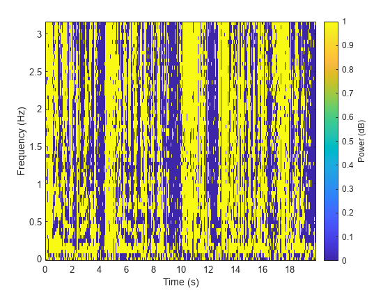
在理想二值掩膜中,掩膜单元值为 0 或 1。如果期望信源的功率大于特定 TF 单元中其他信源合并后的功率,则该单元设置为 1。否则,单元设置为 0。
计算男性说话者的理想二值掩膜,然后将其可视化。
P_M = stft(mSpeech,Window=win,OverlapLength=overlapLength,FFTLength=fftLength,FrequencyRange="onesided");
P_F = stft(fSpeech,Window=win,OverlapLength=overlapLength,FFTLength=fftLength,FrequencyRange="onesided");
[P_mix,F] = stft(mix,Window=win,OverlapLength=overlapLength,FFTLength=fftLength,FrequencyRange="onesided");

binaryMask = abs(P_M) >= abs(P_F);

figure
plotMask(binaryMask,windowLength - overlapLength,F,Fs)
通过将混音 STFT 乘以男性说话者的二值掩膜来估计男性语音的 STFT。通过将混音 STFT 乘以男性说话者的二值掩膜的倒数来估计女性语音的 STFT。
P_M_Hard = P_mix.*binaryMask;
P_F_Hard = P_mix.*(1-binaryMask);
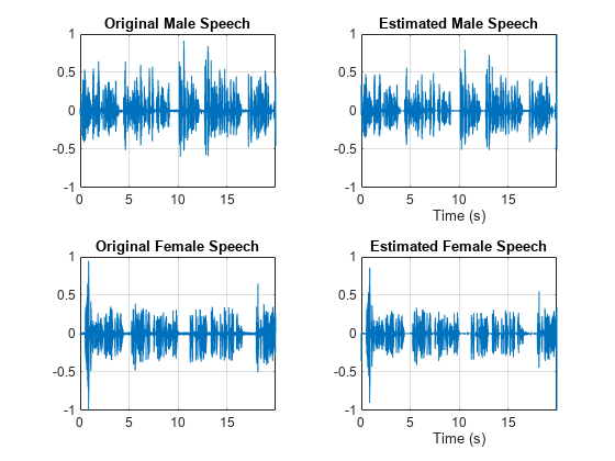
使用逆短时 FFT (ISTFT) 估计男性和女性音频信号。可视化估计的信号和原始信号。收听估计的男性和女性语音信号。
mSpeech_Hard = istft(P_M_Hard,Window=win,OverlapLength=overlapLength,FFTLength=fftLength,FrequencyRange="onesided");
fSpeech_Hard = istft(P_F_Hard,Window=win,OverlapLength=overlapLength,FFTLength=fftLength,FrequencyRange="onesided");

figure
tiledlayout(2,2)

nexttile
plot(t,mSpeech)
axis([t(1) t(end) -1 1])
title("Original Male Speech")
grid on

nexttile
plot(t,mSpeech_Hard)
axis([t(1) t(end) -1 1])
xlabel("Time (s)")
title("Estimated Male Speech")
grid on

nexttile
plot(t,fSpeech)
axis([t(1) t(end) -1 1])
title("Original Female Speech")
grid on

nexttile
plot(t,fSpeech_Hard)
axis([t(1) t(end) -1 1])
title("Estimated Female Speech")
xlabel("Time (s)")
grid on
sound(mSpeech_Hard,Fs)
sound(fSpeech_Hard,Fs)
使用理想软掩膜的信源分离
在软掩膜中,TF 掩膜单元值等于期望的信源功率与总混合功率的比率。TF 单元的值在 [0,1] 范围内。
计算男性说话者的软掩膜。通过将混音 STFT 乘以男性说话者的软掩膜来估计男性说话者的 STFT。通过将混音 STFT 乘以女性说话者的软掩膜来估计女性说话者的 STFT。
使用 ISTFT 估计男性和女性音频信号。
softMask = abs(P_M)./(abs(P_F) + abs(P_M) + eps);

P_M_Soft = P_mix.*softMask;
P_F_Soft = P_mix.*(1-softMask);

mSpeech_Soft = istft(P_M_Soft,Window=win,OverlapLength=overlapLength,FFTLength=fftLength,FrequencyRange="onesided");
fSpeech_Soft = istft(P_F_Soft,Window=win,OverlapLength=overlapLength,FFTLength=fftLength,FrequencyRange="onesided");
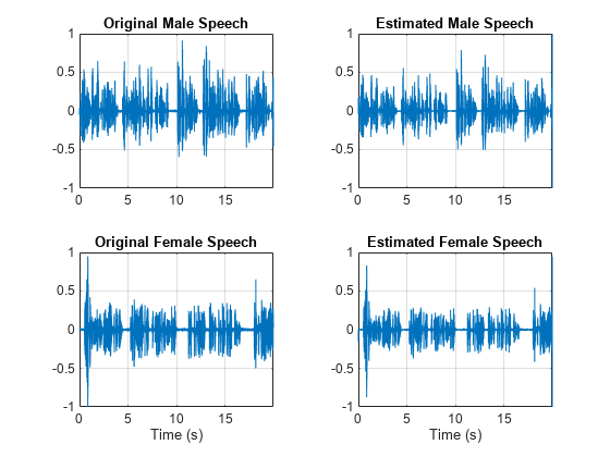
可视化估计的信号和原始信号。收听估计的男性和女性语音信号。请注意,结果非常好,因为掩膜是在完全了解分离的男女音频信号的情况下创建的。
figure
tiledlayout(2,2)

nexttile
plot(t,mSpeech)
axis([t(1) t(end) -1 1])
title("Original Male Speech")
grid on

nexttile
plot(t,mSpeech_Soft)
axis([t(1) t(end) -1 1])
title("Estimated Male Speech")
grid on

nexttile
plot(t,fSpeech)
axis([t(1) t(end) -1 1])
xlabel("Time (s)")
title("Original Female Speech")
grid on

nexttile
plot(t,fSpeech_Soft)
axis([t(1) t(end) -1 1])
xlabel("Time (s)")
title("Estimated Female Speech")
grid on
sound(mSpeech_Soft,Fs)
sound(fSpeech_Soft,Fs)
使用深度学习的掩膜估计
本示例中深度学习网络的目标是估计上述的理想软掩膜。网络估计对应于男性说话者的掩膜。女性说话者的掩膜直接派生自男性掩膜。
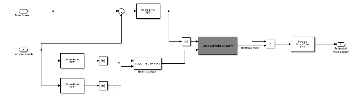
基本的深度学习训练方案如下所示。预测变量是混合(男性 + 女性)音频的幅值频谱。目标是与男性说话者对应的理想软掩膜。回归网络使用预测变量输入来最小化其输出和输入目标之间的均方误差。在输出端,使用输出幅值频谱和混音信号的相位将音频 STFT 转换回时域。
您可以使用短时傅里叶变换 (STFT) 将音频变换为频域,使用的窗长度为 128 个样本、重叠部分为 127 个样本并使用汉宁窗。通过丢弃对应于负频率的频率样本,可以将频谱向量的大小减小到 65(因为时域语音信号是实信号,这样不会导致任何信息丢失)。预测变量输入由 20 个连续的 STFT 向量组成。输出为一个 65×20 软掩膜。
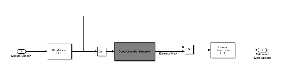
您使用经过训练的网络来估计男性语音。经过训练的网络的输入是混合(男性 + 女性)语音音频。
STFT 目标和预测变量
本节说明如何从训练数据集中生成目标和预测变量信号。
读入分别来自男性和女性说话者的约 400 秒语音的训练信号,采样频率为 4 kHz。低采样率用于加快训练速度。裁剪训练信号使其长度相同。
mSpeechTrain = audioread(fullfile(dataset,"MaleSpeech-16-4-mono-405secs.wav"));
fSpeechTrain = audioread(fullfile(dataset,"FemaleSpeech-16-4-mono-405secs.wav"));

L = min(length(mSpeechTrain),length(fSpeechTrain));
mSpeechTrain = mSpeechTrain(1:L);
fSpeechTrain = fSpeechTrain(1:L);
读入验证信号,该信号由分别来自男性和女性说话者的约 20 秒的语音组成,采样频率为 4 kHz。裁剪验证信号使其长度相同。
mSpeechValidate = audioread(fullfile(dataset,"MaleSpeech-16-4-mono-20secs.wav"));
fSpeechValidate = audioread(fullfile(dataset,"FemaleSpeech-16-4-mono-20secs.wav"));

L = min(length(mSpeechValidate),length(fSpeechValidate));
mSpeechValidate = mSpeechValidate(1:L);
fSpeechValidate = fSpeechValidate(1:L);
将训练信号缩放到相同的功率。将验证信号缩放到相同的功率。
mSpeechTrain = mSpeechTrain/norm(mSpeechTrain);
fSpeechTrain = fSpeechTrain/norm(fSpeechTrain);
ampAdj = max(abs([mSpeechTrain;fSpeechTrain]));

mSpeechTrain = mSpeechTrain/ampAdj;
fSpeechTrain = fSpeechTrain/ampAdj;

mSpeechValidate = mSpeechValidate/norm(mSpeechValidate);
fSpeechValidate = fSpeechValidate/norm(fSpeechValidate);
ampAdj = max(abs([mSpeechValidate;fSpeechValidate]));

mSpeechValidate = mSpeechValidate/ampAdj;
fSpeechValidate = fSpeechValidate/ampAdj;
创建训练和验证“鸡尾酒会”混音。
mixTrain = mSpeechTrain + fSpeechTrain;
mixTrain = mixTrain/max(mixTrain);

mixValidate = mSpeechValidate + fSpeechValidate;
mixValidate = mixValidate/max(mixValidate);
生成训练 STFT。
windowLength = 128;
fftLength = 128;
overlapLength = 128-1;
Fs = 4000;
win = hann(windowLength,"periodic");

P_mix0 = abs(stft(mixTrain,Window=win,OverlapLength=overlapLength,FFTLength=fftLength,FrequencyRange="onesided"));
P_M = abs(stft(mSpeechTrain,Window=win,OverlapLength=overlapLength,FFTLength=fftLength,FrequencyRange="onesided"));
P_F = abs(stft(fSpeechTrain,Window=win,OverlapLength=overlapLength,FFTLength=fftLength,FrequencyRange="onesided"));
对混音 STFT 取对数。通过均值和标准差对这些值进行归一化。
P_mix = log(P_mix0 + eps);
MP = mean(P_mix(:));
SP = std(P_mix(:));
P_mix = (P_mix - MP)/SP;
生成验证 STFT。对混音 STFT 取对数。通过均值和标准差对这些值进行归一化。
P_Val_mix0 = stft(mixValidate,Window=win,OverlapLength=overlapLength,FFTLength=fftLength,FrequencyRange="onesided");
P_Val_M = abs(stft(mSpeechValidate,Window=win,OverlapLength=overlapLength,FFTLength=fftLength,FrequencyRange="onesided"));
P_Val_F = abs(stft(fSpeechValidate,Window=win,OverlapLength=overlapLength,FFTLength=fftLength,FrequencyRange="onesided"));

P_Val_mix = log(abs(P_Val_mix0) + eps);
MP = mean(P_Val_mix(:));
SP = std(P_Val_mix(:));
P_Val_mix = (P_Val_mix - MP) / SP;
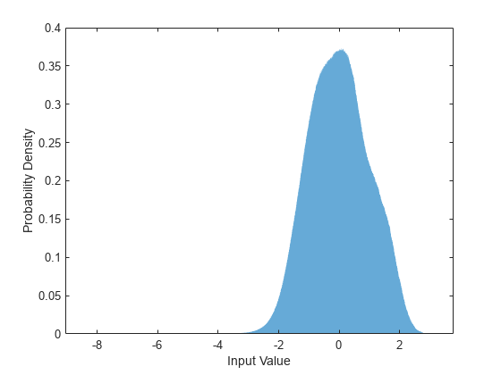
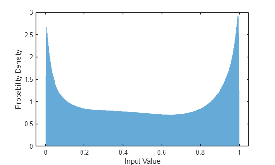
当网络的输入经过归一化且具有适度平滑的分布时,最易于训练神经网络。要检查数据分布是否平滑,请绘制训练数据的 STFT 值的直方图。
figure
histogram(P_mix,EdgeColor="none",Normalization="pdf")
xlabel("Input Value")
ylabel("Probability Density")
计算训练软掩膜。在训练网络时,使用此掩膜作为目标信号。
maskTrain = P_M./(P_M + P_F + eps);
计算验证软掩膜。使用此掩膜评估由经过训练的网络发出的掩膜。
maskValidate = P_Val_M./(P_Val_M + P_Val_F + eps);
要检查目标数据分布是否平滑,请绘制训练数据封装值的直方图。
figure

histogram(maskTrain,EdgeColor="none",Normalization="pdf")
xlabel("Input Value")
ylabel("Probability Density")
根据预测变量和目标信号创建大小为 (65, 20) 的块。为了获得更多训练样本,在连续块之间使用 10 个段作为重叠量。
seqLen = 20;
seqOverlap = 10;
mixSequences = zeros(1 + fftLength/2,seqLen,1,0);
maskSequences = zeros(1 + fftLength/2,seqLen,1,0);

loc = 1;
while loc < size(P_mix,2) - seqLen
    mixSequences(:,:,:,end+1) = P_mix(:,loc:loc+seqLen-1);
    maskSequences(:,:,:,end+1) = maskTrain(:,loc:loc+seqLen-1);
    loc = loc + seqOverlap;
end
根据验证预测变量和目标信号创建大小为 (65,20) 的块。
mixValSequences = zeros(1 + fftLength/2,seqLen,1,0);
maskValSequences = zeros(1 + fftLength/2,seqLen,1,0);
seqOverlap = seqLen;

loc = 1;
while loc < size(P_Val_mix,2) - seqLen
    mixValSequences(:,:,:,end+1) = P_Val_mix(:,loc:loc+seqLen-1);
    maskValSequences(:,:,:,end+1) = maskValidate(:,loc:loc+seqLen-1);
    loc = loc + seqOverlap;
end
重构训练和验证信号。
mixSequencesT = reshape(mixSequences,[1 1 (1 + fftLength/2)*seqLen size(mixSequences,4)]);
mixSequencesV = reshape(mixValSequences,[1 1 (1 + fftLength/2)*seqLen size(mixValSequences,4)]);
maskSequencesT = reshape(maskSequences,[1 1 (1 + fftLength/2)*seqLen size(maskSequences,4)]);
maskSequencesV = reshape(maskValSequences,[1 1 (1 + fftLength/2)*seqLen size(maskValSequences,4)]);
定义深度学习网络
定义网络的各层。将输入大小指定为 1×1×1300 大小的图像。定义两个隐藏的全连接层,每个层有 1300 个神经元。每个隐藏的全连接层后跟一个有偏置的 sigmoid 层。批量归一化层对输出的均值和标准差进行归一化。添加一个包含 1300 个神经元的全连接层。
numNodes = (1 + fftLength/2)*seqLen;

layers = [ ...

    imageInputLayer([1 1 (1 + fftLength/2)*seqLen],Normalization="None")

    fullyConnectedLayer(numNodes)
    BiasedSigmoidLayer(6)
    batchNormalizationLayer
    dropoutLayer(0.1)

    fullyConnectedLayer(numNodes)
    BiasedSigmoidLayer(6)
    batchNormalizationLayer
    dropoutLayer(0.1)

    fullyConnectedLayer(numNodes)
    BiasedSigmoidLayer(0)

    ];
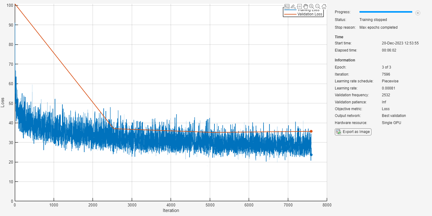
指定网络的训练选项。将 MaxEpochs 设置为 3 以便基于训练数据对网络进行 3 轮训练。将 MiniBatchSize 设置为 64 以便网络可以一次查看 64 个训练信号。将 Plots 设置为 training-progress 以生成显示训练进度随着迭代次数增加而变化的图。将 Verbose 设置为 false 以禁止将对应于图中所示数据的表输出打印到命令行窗口中。将 Shuffle 设置为 every-epoch 以在每轮开始时对训练序列进行乱序处理。将 LearnRateSchedule 设置为 piecewise 以便每经过一定数量的轮次 (1) 后,按指定的因子 (0.1) 降低学习率。将 ValidationData 设置为验证预测变量和目标。设置 ValidationFrequency 以便每轮计算一次验证均方误差。此示例使用自适应矩估计 (ADAM) 求解器。
maxEpochs = 3;
miniBatchSize = 64;

options = trainingOptions("adam", ...
    MaxEpochs=maxEpochs, ...
    MiniBatchSize=miniBatchSize, ...
    SequenceLength="longest", ...
    Shuffle="every-epoch", ...
    Verbose=0, ...
    Plots="training-progress", ...
    ValidationFrequency=floor(size(mixSequencesT,4)/miniBatchSize), ...
    ValidationData={mixSequencesV,permute(maskSequencesV,[4 3 1 2])}, ...
    LearnRateSchedule="piecewise", ...
    LearnRateDropFactor=0.9, ...
    LearnRateDropPeriod=1);
训练深度学习网络
使用 trainnet 以指定的训练选项和层架构训练网络。由于训练集很大,训练过程可能需要几分钟。要加载预训练的网络,请将 speedupExample 设置为 true。
speedupExample =false; if ~speedupExample lossFcn = @(Y,T)0.5*l2loss(Y,T,NormalizationFactor="batch-size"); CocktailPartyNet = trainnet(mixSequencesT,permute(maskSequencesT,[4 3 1 2]),layers,lossFcn,options); else s = load(fullfile(dataset,"CocktailPartyNet.mat")); CocktailPartyNet = s.CocktailPartyNet; end
将验证预测变量传递给网络。输出是估计的掩膜。重构估计的掩膜。
estimatedMasks0 = predict(CocktailPartyNet,mixSequencesV);

estimatedMasks0 = estimatedMasks0.';
estimatedMasks0 = reshape(estimatedMasks0,1 + fftLength/2,numel(estimatedMasks0)/(1 + fftLength/2));
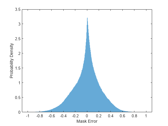
评估深度学习网络
绘制实际掩膜和预期掩膜之间误差的直方图。
figure
histogram(maskValSequences(:) - estimatedMasks0(:),EdgeColor="none",Normalization="pdf")
xlabel("Mask Error")
ylabel("Probability Density")
评估软掩膜估计
估计男声和女声软掩膜。通过为软掩膜设置阈值来估计男声和女声二值掩膜。
SoftMaleMask = estimatedMasks0;
SoftFemaleMask = 1 - SoftMaleMask;
缩短混音 STFT 以匹配估计的掩膜的大小。
P_Val_mix0 = P_Val_mix0(:,1:size(SoftMaleMask,2));
将混音 STFT 乘以男声软掩膜,得到估计的男性语音 STFT。
P_Male = P_Val_mix0.*SoftMaleMask;
使用 ISTFT 获得估计的男性音频信号。缩放音频。
maleSpeech_est_soft = istft(P_Male,Window=win,OverlapLength=overlapLength,FFTLength=fftLength,FrequencyRange="onesided",ConjugateSymmetric=true);
maleSpeech_est_soft = maleSpeech_est_soft/max(abs(maleSpeech_est_soft));
确定要分析的范围和关联的时间向量。
range = windowLength:numel(maleSpeech_est_soft)-windowLength;
t = range*(1/Fs);
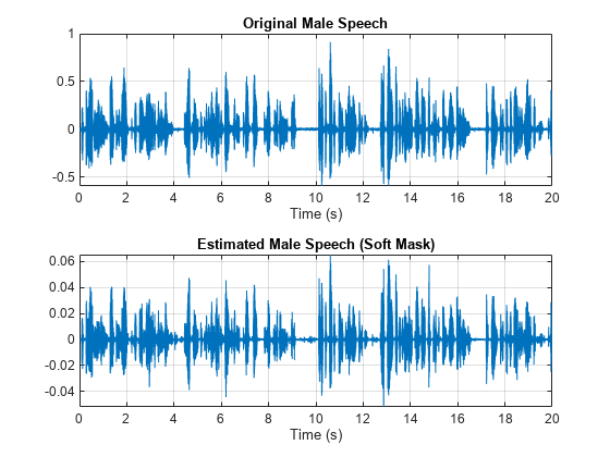
可视化估计的和原始的男性语音信号。收听估计的软掩膜男性语音。
sound(maleSpeech_est_soft(range),Fs)

figure
tiledlayout(2,1)

nexttile
plot(t,mSpeechValidate(range))
title("Original Male Speech")
xlabel("Time (s)")
grid on

nexttile
plot(t,maleSpeech_est_soft(range))
xlabel("Time (s)")
title("Estimated Male Speech (Soft Mask)")
grid on
将混音 STFT 乘以女性软掩膜,得到估计的女性语音 STFT。使用 ISTFT 获得估计的男性音频信号。缩放音频。
P_Female = P_Val_mix0.*SoftFemaleMask;
femaleSpeech_est_soft = istft(P_Female,Window=win,OverlapLength=overlapLength,FFTLength=fftLength,FrequencyRange="onesided",ConjugateSymmetric=true);
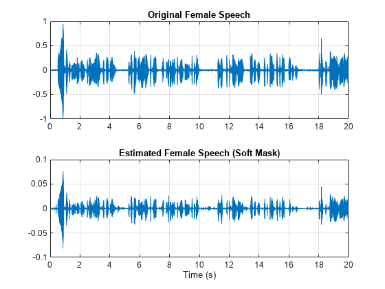
femaleSpeech_est_soft = femaleSpeech_est_soft/max(femaleSpeech_est_soft);可视化估计的和原始的女性语音信号。收听估计的女性语音。
sound(femaleSpeech_est_soft(range),Fs)

figure
tiledlayout(2,1)

nexttile
plot(t,fSpeechValidate(range))
title("Original Female Speech")
grid on

nexttile
plot(t,femaleSpeech_est_soft(range))
xlabel("Time (s)")
title("Estimated Female Speech (Soft Mask)")
grid on
评估二值掩膜估计
通过为软掩膜设置阈值来估计男声和女声二值掩膜。
HardMaleMask = SoftMaleMask >= 0.5;
HardFemaleMask = SoftMaleMask < 0.5;
将混音 STFT 乘以男声二值掩膜,得到估计的男性语音 STFT。使用 ISTFT 获得估计的男性音频信号。缩放音频。
P_Male = P_Val_mix0.*HardMaleMask;
maleSpeech_est_hard = istft(P_Male,Window=win,OverlapLength=overlapLength,FFTLength=fftLength,FrequencyRange="onesided",ConjugateSymmetric=true);
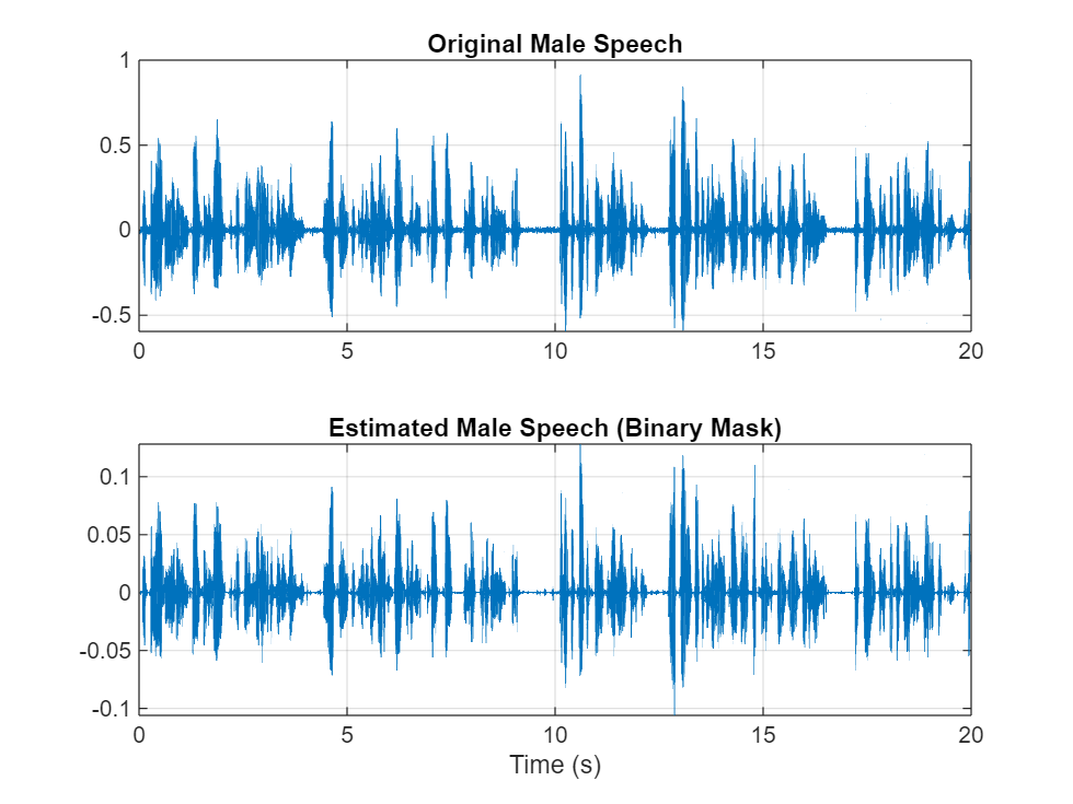
maleSpeech_est_hard = maleSpeech_est_hard/max(maleSpeech_est_hard);可视化估计的和原始的男性语音信号。收听估计的二值掩膜男性语音。
sound(maleSpeech_est_hard(range),Fs)

figure
tiledlayout(2,1)

nexttile
plot(t,mSpeechValidate(range))
title("Original Male Speech")
grid on

nexttile
plot(t,maleSpeech_est_hard(range))
xlabel("Time (s)")
title("Estimated Male Speech (Binary Mask)")
grid on
将混音 STFT 乘以女声二值掩膜,得到估计的男性语音 STFT。使用 ISTFT 获得估计的男性音频信号。缩放音频。
P_Female = P_Val_mix0.*HardFemaleMask;
femaleSpeech_est_hard = istft(P_Female,Window=win,OverlapLength=overlapLength,FFTLength=fftLength,FrequencyRange="onesided",ConjugateSymmetric=true);
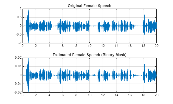
femaleSpeech_est_hard = femaleSpeech_est_hard/max(femaleSpeech_est_hard);可视化估计的和原始的女性语音信号。收听估计的女性语音。
sound(femaleSpeech_est_hard(range),Fs)

figure
tiledlayout(2,1)

nexttile
plot(t,fSpeechValidate(range))
title("Original Female Speech")
grid on

nexttile
plot(t,femaleSpeech_est_hard(range))
title("Estimated Female Speech (Binary Mask)")
grid on
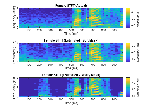
对混音、原始女性语音和男性语音以及估计的女性和男性语音,分别比较其一秒语音段的 STFT。
range = 7e4:7.4e4;

figure
stft(mixValidate(range),Fs,Window=win,OverlapLength=64,FFTLength=fftLength,FrequencyRange="onesided");
title("Mix STFT")
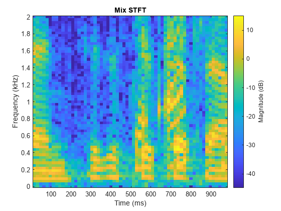
figure
tiledlayout(3,1)

nexttile
stft(mSpeechValidate(range),Fs,Window=win,OverlapLength=64,FFTLength=fftLength,FrequencyRange="onesided");
title("Male STFT (Actual)")

nexttile
stft(maleSpeech_est_soft(range),Fs,Window=win,OverlapLength=64,FFTLength=fftLength,FrequencyRange="onesided");
title("Male STFT (Estimated - Soft Mask)")

nexttile
stft(maleSpeech_est_hard(range),Fs,Window=win,OverlapLength=64,FFTLength=fftLength,FrequencyRange="onesided");
title("Male STFT (Estimated - Binary Mask)");
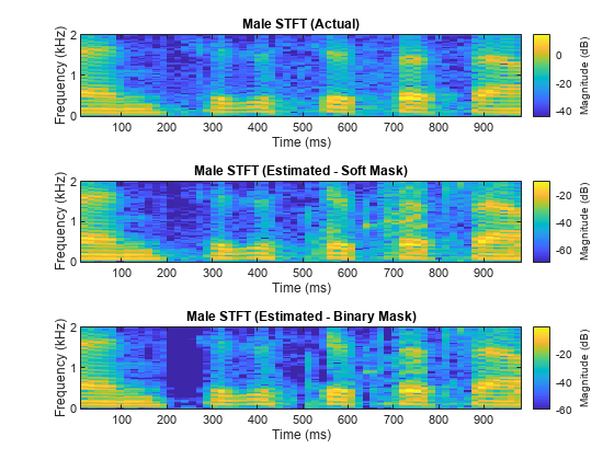
figure
tiledlayout(3,1)

nexttile
stft(fSpeechValidate(range),Fs,Window=win,OverlapLength=64,FFTLength=fftLength,FrequencyRange="onesided");
title("Female STFT (Actual)")

nexttile
stft(femaleSpeech_est_soft(range),Fs,Window=win,OverlapLength=64,FFTLength=fftLength,FrequencyRange="onesided");
title("Female STFT (Estimated - Soft Mask)")

nexttile
stft(femaleSpeech_est_hard(range),Fs,Window=win,OverlapLength=64,FFTLength=fftLength,FrequencyRange="onesided");
title("Female STFT (Estimated - Binary Mask)")
参考资料
[1] "Probabilistic Binary-Mask Cocktail-Party Source Separation in a Convolutional Deep Neural Network", Andrew J.R. Simpson, 2015.
另请参阅
trainnet | trainingOptions | dlnetwork