Denoise Complex-Valued Signal Using Multilayer Perceptron

Since R2026a

This example shows how to create and train a complex-valued neural network for denoising complex-valued signals.

Signal denoising is a fundamental task in signal processing, with applications ranging from communications and radar systems to biomedical signal analysis and audio enhancement. Signals are often corrupted by noise during acquisition or transmission, making it essential to recover the underlying clean signal for accurate analysis and interpretation.

In many applications, signals are represented as complex numbers. In this example, first generate a set of synthetic, complex-valued, noisy signals. Then, create and train a deep learning network that takes a noisy, complex-valued signal and returns a denoised, complex-valued signal.

For an example showing how to train a real-valued neural network to make predictions on complex-valued data by first splitting the signal into its real and imaginary parts, see Train Network with Complex-Valued Data.

Generate Data

Generate a synthetic dataset of 10,000 complex sinusoids.

numSamples = 10000;
signalLength = 100;

For each signal, randomly generate frequency, phase, and amplitude.

frequency = 0.1 + 5*rand(numSamples,1);
phase = 2*pi*rand(numSamples,1);
amplitude = 1 + 10*rand(numSamples,1);

Create time t and noiseless signals cleanSignal.

t = linspace(0,1,signalLength);
cleanSignal = amplitude .* exp(1i*(2*pi*frequency*t + phase));

To create the corresponding noisy signals, add random noise to each signal. Make the noise complex by using the like name-value argument of the randn function.

noiseToAmplitudeRatio = 0.2;
noise = noiseToAmplitudeRatio * amplitude * randn(size(t),like=1j);
noisySignal = cleanSignal + noise;

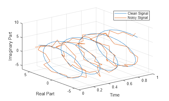
Illustrate a sample clean signal and its corresponding noisy signal by creating a 3-D line plot using the plot3 function.

figure
idx = 1;
hold on
plot3(t,real(cleanSignal(idx,:)),imag(cleanSignal(idx,:)))
plot3(t,real(noisySignal(idx,:)),imag(noisySignal(idx,:)))
legend(["Clean Signal","Noisy Signal"])
xlabel("Time")
ylabel("Real Part")
zlabel("Imaginary Part")
hold off
grid on
view(3)

Figure contains an axes object. The axes object with xlabel Time, ylabel Real Part contains 2 objects of type line. These objects represent Clean Signal, Noisy Signal.

Divide the data into training, validation, and testing data sets by using the trainingPartitions function, which is attached to this example as a supporting function.

[idxTrain,idxValidation,idxTest] = trainingPartitions(numSamples,[0.7,0.15,0.15]);

XTrain = noisySignal(idxTrain,:);
TTrain = cleanSignal(idxTrain,:);

XValidation = noisySignal(idxValidation,:);
TValidation = cleanSignal(idxValidation,:);

XTest = noisySignal(idxTest,:);
TTest = cleanSignal(idxTest,:);

Define Network Architecture

Define a complex-valued multi-layer perceptron architecture. Alternate complexFullyConnectedLayer objects with 512 hidden units with complexReluLayer objects. To output signals, end the network with a complex fully connected layer with output size signalLength.

hiddenSize = 512;
layers = [
    featureInputLayer(signalLength)
    complexFullyConnectedLayer(hiddenSize)
    complexReluLayer
    complexFullyConnectedLayer(hiddenSize)
    complexReluLayer
    complexFullyConnectedLayer(hiddenSize)
    complexReluLayer
    complexFullyConnectedLayer(signalLength)
    ];
net = dlnetwork(layers);

Specify Training Options

Specify the training options. Choosing training options requires empirical analysis. To explore different training option configurations by running experiments, you can use the Experiment Manager app. For this example:

Train using the Adam solver.
Train for 10 epochs.
Shuffle the training data every epoch.
Specify the validation data.
Display the training progress in a plot.
Disable the verbose output.

options = trainingOptions("adam", ...
    MaxEpochs=10, ...
    Shuffle="every-epoch", ...
    ValidationData={XValidation,TValidation}, ...
    Plots="training-progress", ...
    Verbose=false);

Train Network

Train the neural network by using the trainnet function.

net = trainnet(XTrain,TTrain,net,"mse",options);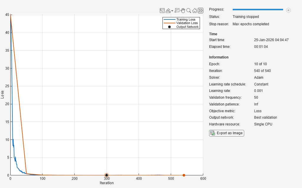

Test Network

Test the network by using the testnet function. Evaluate the mean squared error of the predictions on the test dataset.

mseTrainedNetwork = testnet(net,XTest,TTest,"mse")

mseTrainedNetwork = 
0.0204

Compare the mean squared error to the mean amplitude of the signals in the test set.

meanAmplitude = mean(amplitude(idxTest));
relativeError = mseTrainedNetwork/meanAmplitude

relativeError = 
0.0034

If the network performs well, the relative error is small.

Plot Denoised Signal

Choose a sample signal from the test set.

idx = 1;
noisySample = XTest(idx,:);
cleanSample = TTest(idx,:);

Denoise the signal by using the trained network.

denoisedSample = predict(net,noisySample);

Extract and plot the real and imaginary parts of the clean, noisy, and denoised signals by using the plotTestSample function, which is defined at the bottom of this example.

plotTestSample(t,cleanSample,noisySample,denoisedSample);

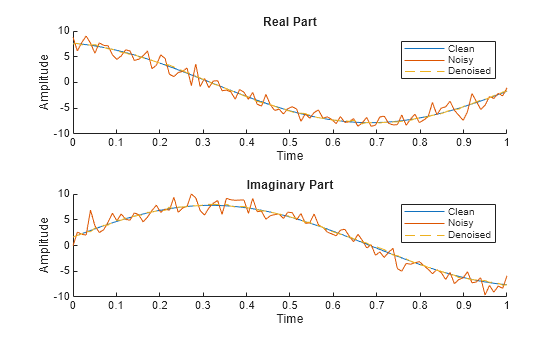
Figure contains 2 axes objects. Axes object 1 with title Real Part, xlabel Time, ylabel Amplitude contains 3 objects of type line. These objects represent Clean, Noisy, Denoised. Axes object 2 with title Imaginary Part, xlabel Time, ylabel Amplitude contains 3 objects of type line. These objects represent Clean, Noisy, Denoised.

The denoised signal is very similar to the original clean signal.

Supporting Functions

The plotTestSample function extracts and plots the real and imaginary parts of the clean, noisy, and denoised signals.

function plotTestSample(t,cleanSample,noisySample,denoisedSample)
realCleanSignal = real(cleanSample);
imagCleanSignal = imag(cleanSample);

realNoisySignal = real(noisySample);
imagNoisySignal = imag(noisySample);

realDenoisedSignal = real(denoisedSample);
imagDenoisedSignal = imag(denoisedSample);

figure
tiledlayout

nexttile
hold on
plot(t,realCleanSignal);
plot(t,realNoisySignal);
plot(t,realDenoisedSignal,"--");
hold off
legend("Clean","Noisy","Denoised");
xlabel("Time");
ylabel("Amplitude");
title("Real Part");

nexttile
hold on
plot(t,imagCleanSignal);
plot(t,imagNoisySignal);
plot(t,imagDenoisedSignal,"--");
hold off
legend("Clean","Noisy","Denoised");
xlabel("Time");
ylabel("Amplitude");
title("Imaginary Part");
end