Evaluate Deep Learning Experiments by Using Metric Functions

Since R2020a

This example shows how to use metric functions to evaluate the results of an experiment. By default, when you run a built-in training experiment, Experiment Manager computes the loss, accuracy (for classification experiments), and root mean squared error (for regression experiments) for each trial in your experiment. To compute other measures, create your own metric function. For example, you can define metric functions to:

Test the prediction performance of a trained network.
Evaluate the training progress by computing the slope of the validation loss over the final epoch.
Display the size of the network used in an experiment that uses different network architectures for each trial.

When each trial finishes training, Experiment Manager evaluates the metric functions and displays their values in the results table.

In this example, you train a network to classify images of handwritten digits. Two metric functions determine how well the trained network identifies the images of the numerals one and seven. For more information on using Experiment Manager to train a network for image classification, see Quickly Set Up Experiment Using Preconfigured Template.

Define Metric Functions

To add a metric function to a built-in training experiment:

In the experiment definition tab, under Metrics, click Add.
In the Add metric dialog box, enter a name for the metric function and click OK. If you enter the name of a function that already exists in the project, Experiment Manager adds it to the experiment. Otherwise, Experiment Manager creates a function defined by a default template.
Select the name of the metric function and click Edit. The metric function opens in MATLAB® Editor.

The input to a metric function is a structure with three fields:

trainedNetwork is the SeriesNetwork object or DAGNetwork object returned by the trainNetwork function. For more information, see net.
trainingInfo is a structure containing the training information returned by the trainNetwork function. For more information, see info.
parameters is a structure with fields from the hyperparameter table.

The output of a custom metric function must be a scalar number, a logical value, or a string.

Open Experiment

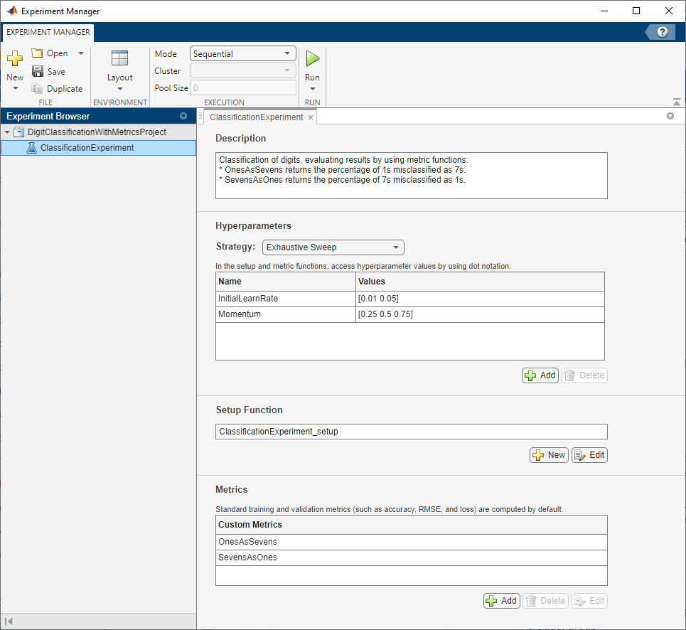
First, open the example. Experiment Manager loads a project with a preconfigured experiment that you can inspect and run. To open the experiment, in the Experiment Browser pane, double-click ClassificationExperiment.

Built-in training experiments consist of a description, a table of hyperparameters, a setup function, and a collection of metric functions to evaluate the results of the experiment. For more information, see Train Network Using trainnet and Display Custom Metrics.

The Description field contains a textual description of the experiment. For this example, the description is:

Classification of digits, evaluating results by using metric functions:
* OnesAsSevens returns the percentage of 1s misclassified as 7s.
* SevensAsOnes returns the percentage of 7s misclassified as 1s.

The Hyperparameters section specifies the strategy and hyperparameter values to use for the experiment. When you run the experiment, Experiment Manager trains the network using every combination of hyperparameter values specified in the hyperparameter table. This example uses the hyperparameters InitialLearnRate and Momentum.

The Setup Function section specifies a function that configures the training data, network architecture, and training options for the experiment. To open this function in MATLAB® Editor, click Edit. The code for the function also appears in Setup Function. The input to the setup function is a structure with fields from the hyperparameter table. The function returns three outputs that you use to train a network for image classification problems. In this example, the setup function has these sections:

Load Training Data defines image datastores that contain the training and validation data. This example loads images from the Digits data set. For more information on this data set, see Image Data Sets.

dataFolder = fullfile(toolboxdir('nnet'), ...
    'nndemos','nndatasets','DigitDataset');
imdsTrain = imageDatastore(dataFolder, ...
    IncludeSubfolders=true, ...
    LabelSource="foldernames");
 
numTrainingFiles = 750;
[imdsTrain,imdsValidation] = splitEachLabel(imdsTrain,numTrainingFiles);

Define Network Architecture defines the architecture for a convolutional neural network for deep learning classification. This example uses the default classification network provided by the setup function template.

inputSize = [28 28 1];
numClasses = 10;
layers = [
    imageInputLayer(inputSize)
    convolution2dLayer(5,20)
    batchNormalizationLayer
    reluLayer
    fullyConnectedLayer(numClasses)
    softmaxLayer
    classificationLayer];

Specify Training Options defines a trainingOptions object for the experiment. The example loads the values for the training options InitialLearnRate and Momentum from the hyperparameter table.

options = trainingOptions("sgdm", ...
    MaxEpochs=5, ... 
    ValidationData=imdsValidation, ...
    ValidationFrequency=30, ...
    InitialLearnRate=params.InitialLearnRate, ...
    Momentum=params.Momentum, ...
    Verbose=false);

The Metrics section specifies optional functions that evaluate the results of the experiment. Experiment Manager evaluates these functions each time it finishes training the network. This example includes two metric functions:

OnesAsSevens returns the percentage of images of the numeral one that the trained network misclassifies as sevens.
SevensAsOnes returns the percentage of images of the numeral seven that the trained network misclassifies as ones.

Each of these functions uses the trained network to classify the entire Digits data set. Then, the functions determine the number of images for which the actual label and the predicted label disagree. For example, the function OnesAsSevens computes the number of images with an actual label of "1" and a predicted label of "7". Similarly, the function SevensAsOnes computes the number of images with an actual label of "7" and a predicted label of "1". To open these functions in MATLAB Editor, select the name of a metric function and click Edit. The code for these functions also appears in Find Ones Misclassified as Sevens and Find Sevens Misclassified as Ones.

Run Experiment

When you run the experiment, Experiment Manager trains the network defined by the setup function six times. Each trial uses a different combination of hyperparameter values. By default, Experiment Manager runs one trial at a time. If you have Parallel Computing Toolbox™, you can run multiple trials at the same time or offload your experiment as a batch job in a cluster:

To run one trial of the experiment at a time, on the Experiment Manager toolstrip, set Mode to Sequential and click Run.
To run multiple trials at the same time, set Mode to Simultaneous and click Run. If there is no current parallel pool, Experiment Manager starts one using the default cluster profile. Experiment Manager then runs as many simultaneous trials as there are workers in your parallel pool. For best results, before you run your experiment, start a parallel pool with as many workers as GPUs. For more information, see Run Experiments in Parallel and GPU Computing Requirements (Parallel Computing Toolbox).
To offload the experiment as a batch job, set Mode to Batch Sequential or Batch Simultaneous, specify your cluster and pool size, and click Run. For more information, see Offload Experiments as Batch Jobs to a Cluster.

A table of results displays the metric function values for each trial.

Evaluate Results

To find the best result for your experiment, sort the table of results. For example, find the trial with the smallest number of misclassified ones:

Point to the OnesAsSevens column.
Click the triangle icon.
Select Sort in Ascending Order.

Similarly, find the trial with the smallest number of misclassified sevens by opening the drop-down menu for the SevensAsOnes column and selecting Sort in Ascending Order.

If no single trial minimizes both values, opt for a trial that ranks well for both metrics. For example, you can export the results table to the MATLAB workspace as a nested table array and compute the average of the two metric values for each trial:

On the Experiment Manager toolstrip, click Export > Results Table.
In the dialog window, enter the name of a workspace variable for the exported table. The default name is resultsTable.
In the MATLAB Command Window, use the exported table as the input to the function averageMetrics:

averageMetrics(resultsTable)

To view the code for this function, see Compute Average Metric Values. The function displays a summary of the metric information for the trial with the lowest average metric value.

******************************************

Best trial: 4
Ones misclassified as sevens: 1.3000% (Ranking: 3)
Sevens misclassified as ones: 1.2000% (Ranking: 1)
Average of metric values: 1.2500%

******************************************

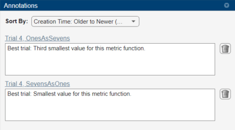
To record observations about the results of your experiment, add an annotation:

In the results table, right-click the OnesAsSevens cell of the best trial.
Select Add Annotation.
In the Annotations pane, enter your observations in the text box.
Repeat the previous steps for the SevensAsOnes cell.

Close Experiment

In the Experiment Browser pane, right-click DigitClassificationWithMetricsProject and select Close Project. Experiment Manager closes the experiment and results contained in the project.

Setup Function

This function configures the training data, network architecture, and training options for the experiment. The input to this function is a structure with fields from the hyperparameter table. The function returns three outputs that you use to train a network for image classification problems.

function [imdsTrain,layers,options] = ClassificationExperiment_setup(params)

Load Training Data

dataFolder = fullfile(toolboxdir('nnet'), ...
    'nndemos','nndatasets','DigitDataset');
imdsTrain = imageDatastore(dataFolder, ...
    IncludeSubfolders=true, ...
    LabelSource="foldernames");
 
numTrainingFiles = 750;
[imdsTrain,imdsValidation] = splitEachLabel(imdsTrain,numTrainingFiles);

Define Network Architecture

inputSize = [28 28 1];
numClasses = 10;
layers = [
    imageInputLayer(inputSize)
    convolution2dLayer(5,20)
    batchNormalizationLayer
    reluLayer
    fullyConnectedLayer(numClasses)
    softmaxLayer
    classificationLayer];

Specify Training Options

options = trainingOptions("sgdm", ...
    MaxEpochs=5, ... 
    ValidationData=imdsValidation, ...
    ValidationFrequency=30, ...
    InitialLearnRate=params.InitialLearnRate, ...
    Momentum=params.Momentum, ...
    Verbose=false);

end

Find Ones Misclassified as Sevens

This function determines the number of ones that are misclassified as sevens.

function metricOutput = OnesAsSevens(trialInfo)

actualValue = "1";
predValue = "7";
 
net = trialInfo.trainedNetwork;
 
dataFolder = fullfile(toolboxdir('nnet'), ...
    'nndemos','nndatasets','DigitDataset');
imds = imageDatastore(dataFolder, ...
    IncludeSubfolders=true, ...
    LabelSource="foldernames");
 
YActual = imds.Labels;
YPred = classify(net,imds);
 
K = sum(YActual == actualValue & YPred == predValue);
N = sum(YActual == actualValue);
 
metricOutput = 100*K/N;
 
end

Find Sevens Misclassified as Ones

This function determines the number of sevens that are misclassified as ones.

function metricOutput = SevensAsOnes(trialInfo)

actualValue = "7";
predValue = "1";
 
net = trialInfo.trainedNetwork;
 
dataFolder = fullfile(toolboxdir('nnet'), ...
    'nndemos','nndatasets','DigitDataset');
imds = imageDatastore(dataFolder, ...
    IncludeSubfolders=true, ...
    LabelSource="foldernames");
 
YActual = imds.Labels;
YPred = classify(net,imds);
 
K = sum(YActual == actualValue & YPred == predValue);
N = sum(YActual == actualValue);
 
metricOutput = 100*K/N;
 
end

Compute Average Metric Values

This function extracts metric values from the results table. The function then appends average metric values and rankings for each metric to the results table, and displays a summary of the metric information for the trial with the smallest average metric value.

function averageMetrics(results)

results = splitvars(results);
metric1 = results.OnesAsSevens;
metric2 = results.SevensAsOnes;
MetricAverage = (metric1+metric2)/2;
 
results = [results table(MetricAverage)];
N = height(results);
 
results = sortrows(results,"OnesAsSevens");
OnesAsSevensRanking = (1:N)';
results = [results table(OnesAsSevensRanking)];
 
results = sortrows(results,"SevensAsOnes");
SevensAsOnesRanking = (1:N)';
results = [results table(SevensAsOnesRanking)];
 
results = sortrows(results,"MetricAverage");
 
fprintf("\n******************************************\n\n");
fprintf("Best trial: %d\n",results.Trial(1));
fprintf("Ones misclassified as sevens: %.4f%% (Ranking: %d)\n", ...
    results.OnesAsSevens(1),results.OnesAsSevensRanking(1));
fprintf("Sevens misclassified as ones: %.4f%% (Ranking: %d)\n", ...
    results.SevensAsOnes(1),results.SevensAsOnesRanking(1));
fprintf("Average of metric values: %.4f%%\n", ...
    results.MetricAverage(1));
fprintf("\n******************************************\n\n");
 
end