Prepare Data for ECG Signal Classification
This example shows how to prepare data for training a deep learning network for electrocardiogram (ECG) signal classification. This example is step two in a series of examples that take you through an ECG signal classification workflow. This example follows the Define Requirements for ECG Signal Classification Using Deep Learning example. For more information about the full workflow, see ECG Signal Classification Using Deep Learning.
To run this example, open ECG Signal Classification Using Deep Learning and navigate to scripts\S2_PrepareData. Alternatively, if you already have MATLAB open, then run
openExample("deeplearning_shared/ECGSignalClassificationUsingDeepLearningExample")This project contains all of the steps for this workflow. You can run the scripts in order or run each one independently.
Data preprocessing converts raw data into a format suitable for deep learning and can improve model performance by enhancing important features or reducing artifacts such as noise.
In this example, you follow these steps to prepare data for training a deep learning-based binary classifier to detect atrial fibrillation:
Split ECG signals into equal-length segments to minimize excessive padding, which can negatively affect network performance.
Downsample ECG signals from 300 Hz to 60 Hz to reduce data size and speed up training.
Divide the data into training and test sets.
Verify that the data meets the requirements defined in Define Requirements for ECG Signal Classification Using Deep Learning.
This example uses ECG data from the PhysioNet 2017 Challenge [1], [2], [3], which is available at https://physionet.org/challenge/2017/. The data consists of a set of ECG signals sampled at 300 Hz and divided by a group of experts into four different classes: Normal (N), Atrial Fibrillation (A), Other Rhythm (O), and Noisy Recording (~). In this example, use only the Normal and Atrial Fibrillation classes.
Load and Examine Data
To download the data from the PhysioNet website and generate a MAT file (PhysionetData.mat) that contains the ECG signals in the appropriate format, run the downloadPhysionetData function. Downloading the data might take a few minutes.
if ~isfile(fullfile(currentProject().RootFolder,"data","PhysionetData.mat"))
    downloadPhysionetData;
end
load PhysionetData
The data contains two variables: Signals and Labels. Signals is a cell array containing the ECG signals. Labels is a categorical array containing the corresponding ground-truth labels of the signals.
Use the summary function to see how many N and A signals the data contains.
summary(Labels)
Labels: 5788×1 categorical

     A                 738
     N                5050
     <undefined>         0
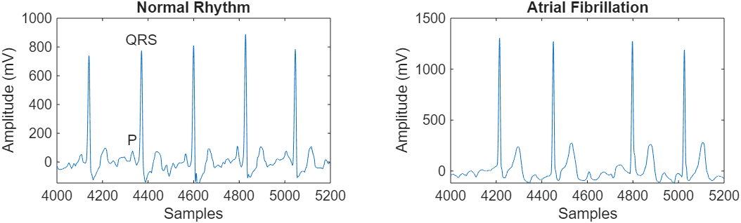
Atrial Fibrillation heartbeats are spaced out at irregular intervals whereas normal heartbeats occur regularly. Atrial Fibrillation heartbeat signals also often lack a P-wave, which pulses before the QRS complex in a Normal heartbeat signal. Visualize a segment of one signal from each class and mark the QRS complex and P-wave.
normal = Signals{1};
aFib = Signals{4};

tiledlayout("flow")

nexttile
plot(normal)
title("Normal Rhythm")
xlim([4000,5200])
xlabel("Samples")
ylabel("Amplitude (mV)")
text(4330,150,"P",HorizontalAlignment="center")
text(4370,850,"QRS",HorizontalAlignment="center")

nexttile
plot(aFib)
title("Atrial Fibrillation")
xlim([4000,5200])
xlabel("Samples")
ylabel("Amplitude (mV)")
Segment Data
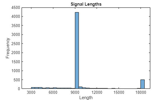
The ECG signals have been sampled at 300 Hz, but the recordings vary in length. Generate a histogram of signal lengths. Most of the signals are 9000 samples long.
Find the length of each signal.
L = zeros(1,numel(Signals));
for i = 1:numel(Signals)
    L(i) = length(Signals{i});
end
Plot the signal lengths.
figure
h = histogram(L);
xticks(0:3000:18000)
xticklabels(0:3000:18000)
title("Signal Lengths")
xlabel("Length")
ylabel("Frequency")
In step three of this workflow, you use the trainnet function to train a deep learning network to classify ECG signals. During training, the trainnet function splits the data into mini-batches. The function then pads or truncates signals in the same mini-batch so they all have the same length. Too much padding or truncating can have a negative effect on the performance of the network because the network might interpret a signal incorrectly based on the added or removed information.
To avoid excessive padding or truncating when you train the network, use the supporting function helperSegmentSignals, which is attached to this project as a supporting function, to segment the ECG signals so that they are at most 9000 samples long. The function ignores signals with fewer than 9000 samples. If a signal has more than 9000 samples, then the helperSegmentSignals function breaks it into as many 9000-sample segments as possible and ignores the remaining samples. For example, a signal with 18500 samples becomes two 9000-sample signals, and the last 500 samples are ignored. This segmentation approach is appropriate for ECG data because the features a network uses to classify a signal as Normal or Atrial Fibrillation are often delocalized in time. This means that even if a long signal is split into multiple segments, each segment can still contain sufficient information for the network to detect signs of atrial fibrillation.
[Signals,Labels] = helperSegmentSignals(Signals,Labels);
View the first five elements of the Signals array to verify that each entry is now 9000 samples long.
Signals(1:5)'
ans=1×5 cell array
    1×9000 double    1×9000 double    1×9000 double    1×9000 double    1×9000 double
Downsample Data
To reduce training time, use the downsample (Signal Processing Toolbox) function to decrease the sample rate by a factor of five.
downSampleFactor = 5;

for i = 1:numel(Signals)
    Signals{i} = downsample(Signals{i},downSampleFactor);
end
View the first five elements of the Signals array to verify that each entry is now 1800 samples long.
Signals(1:5)'
ans=1×5 cell array
    1×1800 double    1×1800 double    1×1800 double    1×1800 double    1×1800 double
Hold Out Data for Testing and Calibration
Split the data into training, calibration, and test sets by using the cvpartition function. Use 70% of the observations for training and reserve 15% each for calibration and testing. You can use the calibration set to calibrate the distribution discriminator. For more information, see step six of this workflow, Out-of-Distribution Detection for ECG Signal Classification.
rng(0)
hpartition = cvpartition(Labels,HoldOut=0.3);

XTrain = Signals(hpartition.training);
TTrain = Labels(hpartition.training);

XTemp = Signals(hpartition.test);
TTemp = Labels(hpartition.test);

hpartition = cvpartition(TTemp,HoldOut=0.5);

XCalib = XTemp(hpartition.training);
TCalib = TTemp(hpartition.training);

XTest = XTemp(hpartition.test);
TTest = TTemp(hpartition.test);
The data is now ready to use to train a deep learning model. To train the model, see Train Deep Learning Network for ECG Signal Classification.
Optionally, if you have Requirements Toolbox™, you can first link and test data requirements.
Verify Data Requirements with MATLAB Tests
If you have Requirements Toolbox™, then you can verify requirements in your project by linking them to tests in the project and running the tests by using the Requirements Editor (Requirements Toolbox). You can then view the requirements verification status in the Requirements Editor.
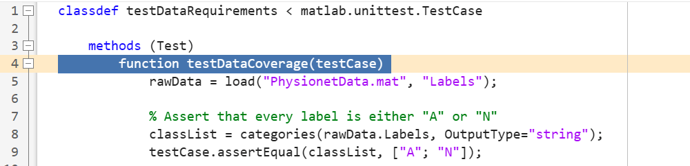
In this example, open the prefilled test file testDataRequirements. The testDataCoverage function checks that the data set contains both "Normal" and "Atrial Fibrillation" labels.
Open the testDataRequirements test file.
edit testDataRequirements.m
Select the function declaration line for the test testDataRequirements.
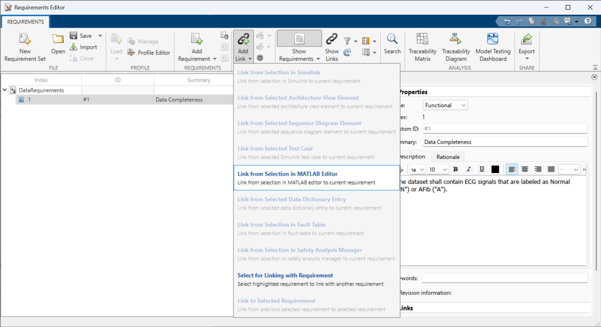
Open the data requirements set in the Requirements Editor. To add columns that indicate the implementation and verification status of the requirements, click Columns and then select Implementation Status and Verification Status.
slreq.open("DataRequirements.slreqx");
Select the Data Completeness requirement.
![]()
In the toolstrip, click Add Link > Link from Selection in MATLAB Editor.
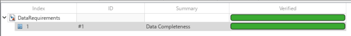
In the Requirements Editor, right-click on the requirements set DataRequirements and click Run Tests. In the Run Tests dialog box, select the testDataCoverage test and click Run Tests. Doing so runs the test linked to the data requirements. If the test passes, then the verification status turns to green.
To document your requirements for review, you can create a report for one or more requirement sets. For general information about how to create reports from requirement sets see Report Requirements Information (Requirements Toolbox).
References
[1] AF Classification from a Short Single Lead ECG Recording: the PhysioNet/Computing in Cardiology Challenge, 2017. https://physionet.org/challenge/2017/
[2] Clifford, Gari, Chengyu Liu, Benjamin Moody, Li-wei H. Lehman, Ikaro Silva, Qiao Li, Alistair Johnson, and Roger G. Mark. "AF Classification from a Short Single Lead ECG Recording: The PhysioNet Computing in Cardiology Challenge 2017." Computing in Cardiology (Rennes: IEEE). Vol. 44, 2017, pp. 1–4.
[3] Goldberger, A. L., L. A. N. Amaral, L. Glass, J. M. Hausdorff, P. Ch. Ivanov, R. G. Mark, J. E. Mietus, G. B. Moody, C.-K. Peng, and H. E. Stanley. "PhysioBank, PhysioToolkit, and PhysioNet: Components of a New Research Resource for Complex Physiologic Signals". Circulation. Vol. 101, No. 23, 13 June 2000, pp. e215–e220. http://circ.ahajournals.org/content/101/23/e215.full
See Also
Requirements Editor (Requirements Toolbox)