Train Deep Learning Network for ECG Signal Classification
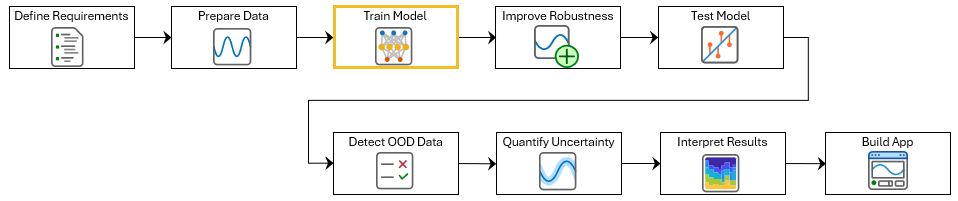
This example shows how to train a deep neural network for ECG signal classification. This example is step three in a series of examples that take you through an ECG signal classification workflow. This example follows the Prepare Data for ECG Signal Classification example. For more information about the full workflow, see ECG Signal Classification Using Deep Learning.
To run this example, open ECG Signal Classification Using Deep Learning and navigate to scripts\S3_TrainNetwork. Alternatively, if you already have MATLAB open, then run
openExample("deeplearning_shared/ECGSignalClassificationUsingDeepLearningExample")This project contains all of the steps for this workflow. You can run the scripts in order or run each one independently.
This example shows how to train a 1-D convolutional neural network (CNN) to classify ECG signals as either normal ("N") or showing signs of atrial fibrillation ("A"). A 1-D convolutional layer learns features by applying sliding convolutional filters to 1-D input. 1-D convolutional layers are often faster than recurrent layers, but they might not capture long-term dependencies as effectively.
Load the training data. If you have run the previous step, Prepare Data for ECG Signal Classification, then the example uses the data that you prepared in that step. Otherwise, the example prepares the data as shown in Prepare Data for ECG Signal Classification.
if ~exist("XTrain","var") || ~exist("TTrain","var")
    [XTrain,TTrain] = prepareECGData;
end
Define Network Architecture
Define the 1-D convolutional neural network architecture.
Specify the input size as 1, since each ECG signal has only one feature.
Specify two blocks of 1-D convolution, ReLU, and layer normalization layers, where the convolutional layer has a filter size of 5. Specify 32 and 64 filters for the first and second convolutional layers, respectively.
To reduce the output of the convolutional layers to a single vector, use a 1-D global average pooling layer.
To map the output to a vector of probabilities, specify a fully connected layer with an output size of 2, followed by a softmax layer.
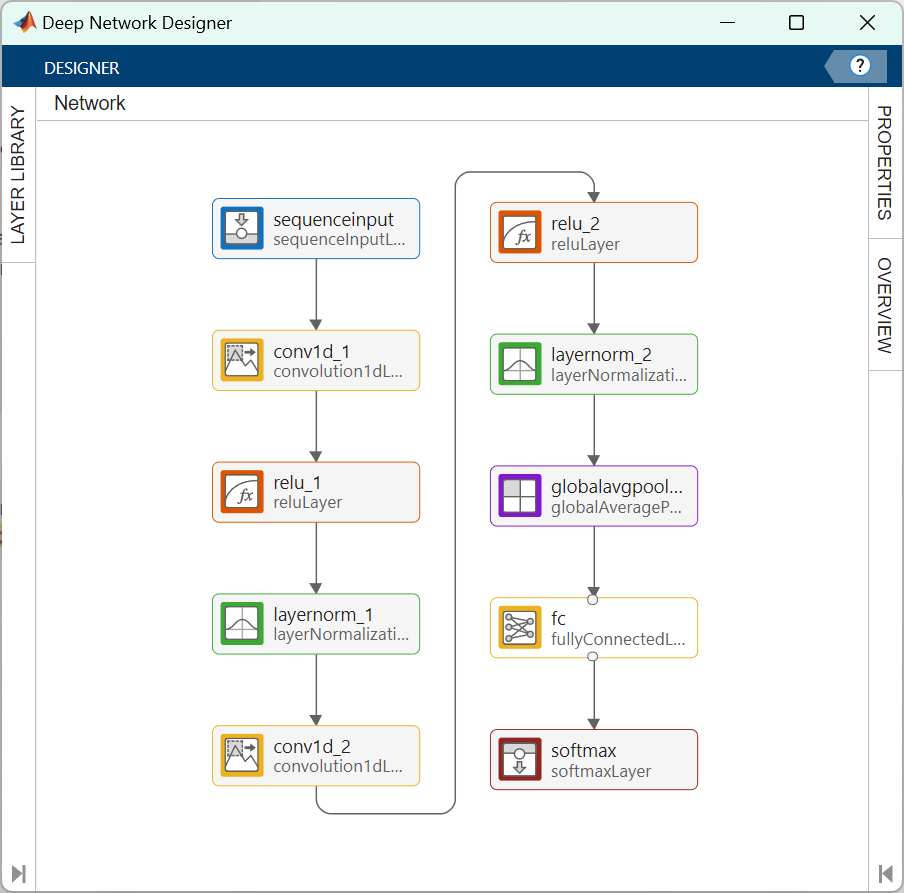
You can also build this network using the Deep Network Designer app. On the Deep Network Designer Start Page, in the Sequence-to-Label Classification Networks (Untrained) section, click 1-D CNN.
numChannels = size(XTrain{1},1);

filterSize = 5;
numFilters = 32;

classNames = categories(TTrain);
numClasses = numel(classNames);

layers = [ ...
    sequenceInputLayer(numChannels)
    convolution1dLayer(filterSize,numFilters,Padding="causal")
    reluLayer
    layerNormalizationLayer
    convolution1dLayer(filterSize,2*numFilters,Padding="causal")
    reluLayer
    layerNormalizationLayer
    globalAveragePooling1dLayer
    fullyConnectedLayer(numClasses)
    softmaxLayer];
You can use the Deep Network Designer app to visualize the network.
deepNetworkDesigner(layers)
Specify Training Options
Specify the training options. Choosing among the options requires empirical analysis. To explore different training option configurations by running experiments, you can use the Experiment Manager app.
Train for 40 epochs using the Adam optimizer with a learn rate of 0.01.
Left pad the sequences.
Monitor the training progress in a plot and suppress the verbose output.
options = trainingOptions("adam", ...
    MaxEpochs=40, ...
    MiniBatchSize=128, ...
    InitialLearnRate=0.01, ...
    SequencePaddingDirection="left", ...
    Plots="training-progress", ...
    Metrics="accuracy", ...
    Verbose=false, ...
    InputDataFormats="CTB", ...
    Shuffle="every-epoch");
Create Custom Loss Function for Imbalanced Classes
When working with imbalanced data sets, classification networks can become biased toward the majority class. The network can achieve high overall classification accuracy by always predicting the majority class, while failing to detect the minority class.
To visualize the class imbalance, plot a histogram of the class frequencies.
histogram(TTrain)
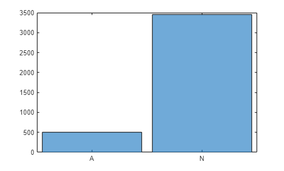
In this example, the training data contains many more normal signals than signals showing signs of atrial fibrillation. Therefore, the predictions of the network might be biased toward the normal class, resulting in more false negatives. This means that patients with atrial fibrillation could be incorrectly classified as healthy and may not receive the necessary care. A network trained on this data would be unlikely to meet the false negative rate requirement.
To prevent the network from being biased towards more prevalent classes, you can calculate class weights that are inversely proportional to the frequency of the classes. These weights scale the loss function during training so that errors made on rare classes contribute more to the overall loss than errors made on common classes. This encourages the network to pay more attention to underrepresented classes.
Calculate class weights that are inversely proportional to the frequency of the classes. For more information on calculating inverse-frequency class weights, see Train Sequence Classification Network Using Data with Imbalanced Classes.
classes = unique(TTrain)';
numClasses = numel(classes);

for i=1:numClasses
    classFrequency(i) = sum(TTrain(:) == classes(i));
    classWeights(i) = numel(XTrain)/(numClasses*classFrequency(i));
end

dictionary(classes,classWeights)
ans =

  dictionary (categorical ⟼ double) with 2 entries:

    A ⟼ 3.9354
    N ⟼ 0.5728
Create a custom loss function that takes predictions Y and targets T and returns the weighted cross-entropy loss.
lossFcn = @(Y,T) crossentropy(Y,T,classWeights, ...
    NormalizationFactor="all-elements", ...
    WeightsFormat="C")*numClasses;
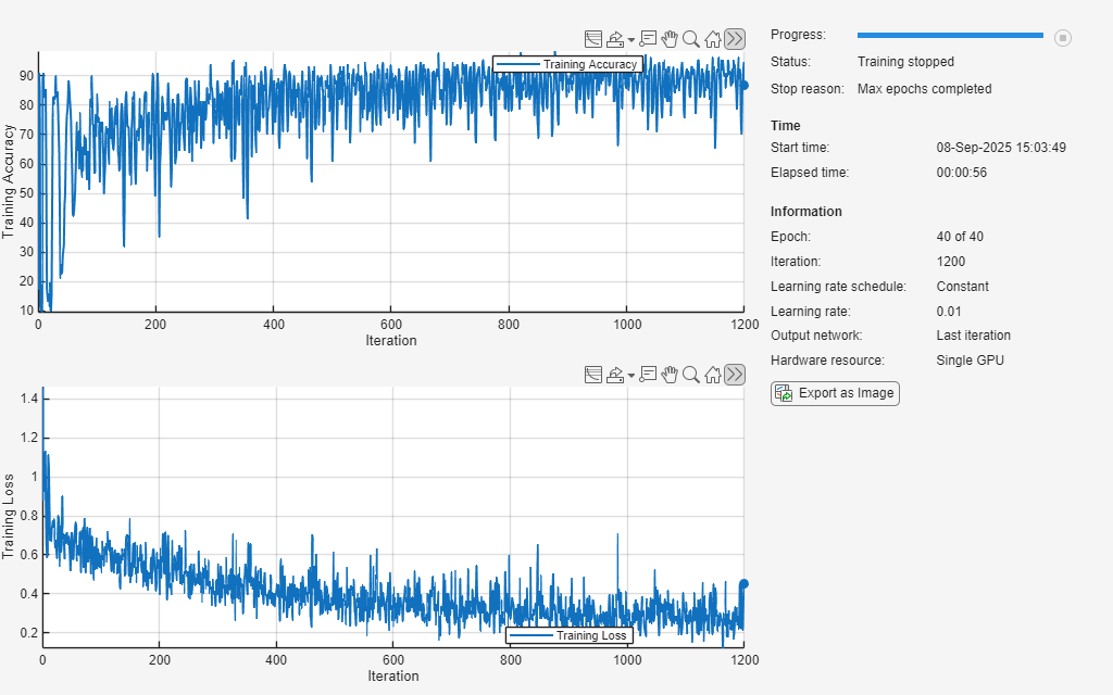
Train Network
Train the convolutional network with the specified options by using the trainnet function. By default, the trainnet function uses a GPU if one is available. Using a GPU requires a Parallel Computing Toolbox™ license and a supported GPU device. For information on supported devices, see GPU Computing Requirements (Parallel Computing Toolbox). Otherwise, the function uses the CPU. To specify the execution environment, use the ExecutionEnvironment training option.
To train the network, set the doTraining flag to true. Otherwise, load a pretrained network.
doTraining =false; if doTraining [net,info] = trainnet(XTrain,TTrain,layers,lossFcn,options); else load("trainedECGNetwork.mat"); show(info) end
Test Network
Load the test data. If you have run Prepare Data for ECG Signal Classification, then the example uses the data that you prepared in that step. Otherwise, the example prepares the data as shown in Prepare Data for ECG Signal Classification.
if ~exist("XTest","var") || ~exist("TTest","var")
    [~,~,~,~,XTest,TTest] = prepareECGData;
end
Test the accuracy of the neural network using the testnet function. By default, the testnet function uses a GPU if one is available. To select the execution environment manually, use the ExecutionEnvironment argument of the testnet function.
accuracy = testnet(net,XTest,TTest,"accuracy",InputDataFormats="CTB")
accuracy =
81.3679
The network performs well on clean data, but it may be vulnerable to adversarial examples. In the next step of the workflow, you retrain the network with adversarial training to improve its robustness.