Improve Adversarial Robustness of Deep Learning Network for ECG Signal Classification

Since R2026a

This example uses:

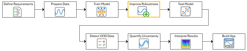
This example shows how to train a more robust deep neural network for ECG signal classification. This example is step four in a series of examples that take you through an ECG signal classification workflow. This example follows the Train Deep Learning Network for ECG Signal Classification example. For more information about the full workflow, see ECG Signal Classification Using Deep Learning.

Diagram of the ECG signal classification workflow with the current step, Improve Robustness, highlighted.

To run this example, open ECG Signal Classification Using Deep Learning and navigate to scripts\S4_TrainRobustNetwork. Alternatively, if you already have MATLAB open, then run

openExample("deeplearning_shared/ECGSignalClassificationUsingDeepLearningExample")

This project contains all of the steps for this workflow. You can run the scripts in order or run each one independently.

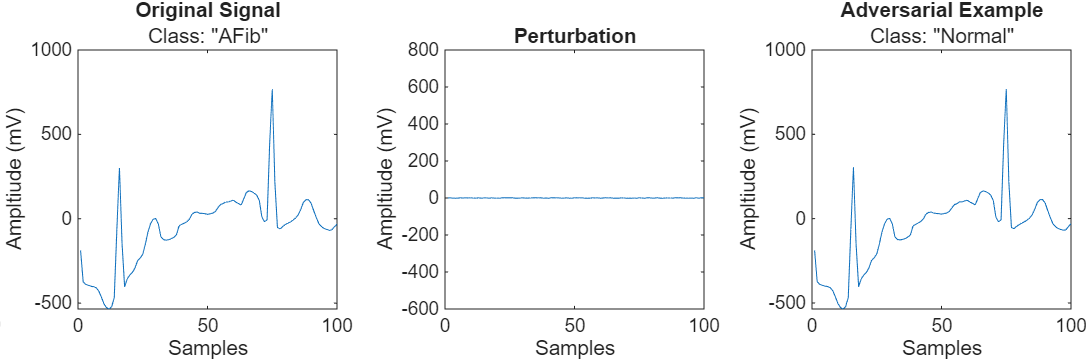
Neural networks can be susceptible to adversarial examples, where very small changes to an input can cause it to be misclassified. These changes are often imperceptible to humans. For example, adding a small perturbation to an atrial fibrillation signal means that the network now classifies it as normal.

Three plots comparing an original AFib signal, a small perturbation, and an adversarial example classified as Normal. The adversarial example looks very similar to the original signal.

A classifier is adversarially robust if the predicted class does not change when the input is perturbed within some specified threshold. This example shows how to use adversarial training to improve the robustness of a pretrained ECG signal classifier.

Load the training data. If you have run the previous step, Prepare Data for ECG Signal Classification, then the example uses the data that you prepared in that step. Otherwise, the example prepares the data as shown in Prepare Data for ECG Signal Classification.

if ~exist("XTrain","var") || ~exist("TTrain","var")
    [XTrain,TTrain] = prepareECGData;
end

Load a pretrained network. If you have run the previous step, Train Deep Learning Network for ECG Signal Classification, then the example uses your trained network. Otherwise, load a pretrained network that has been trained using the steps shown in Train Deep Learning Network for ECG Signal Classification.

if ~exist("net","var")
    load("trainedECGNetwork.mat");
end

Generate Adversarial Examples

You can generate adversarial examples by using the findAdversarialExamples function. For more information about generating adversarial examples, see Generate Untargeted and Targeted Adversarial Examples for Image Classification.

Set a maximum perturbation size of 10. Create lower and upper bounds for each of the training signals. The bounds determine the range within which the adversarial examples can be found.

maxPerturbation = 10;

XTrainAdv = cell2mat(XTrain);
XTrainAdv = dlarray(XTrainAdv,"BTC");

XLower = XTrainAdv - maxPerturbation;
XUpper = XTrainAdv + maxPerturbation;

Specify the adversarial options. Use the adversarialOptions function to select the Fast Gradient Sign Method (FGSM) with a step size of 10. FGSM is a method of finding adversarial examples.

advOpts = adversarialOptions("fgsm",StepSize=10,Verbose=true);

Generate adversarial examples using the findAdversarialExamples function. Set the random seed for reproducibility.

rng(0)
gpurng(0)
[example,mislabel,iX] = findAdversarialExamples(net,XLower,XUpper,TTrain,Algorithm=advOpts);

Number of mini-batches to process: 31
..........   ..........   ..........   . (31 mini-batches)
Total time = 1.8 seconds.

Plot an adversarial example and the ECG signal the function generated it from side-by-side. The adversarial example looks almost identical to the original signal, but the network misclassifies it.

figure
tiledlayout(2,1)

nexttile
plot(XTrain{iX(1)})
title("Original Signal (" + "Label: " + string(TTrain(iX(1)))+ ")")
xlabel("Samples")
ylabel("Amplitude (mV)")

nexttile
plot(squeeze(example(:,1,:)))
title("Adversarial Example (" + "Mislabel: " + string(mislabel(:,1)) + ")")
xlabel("Samples")
ylabel("Amplitude (mV)")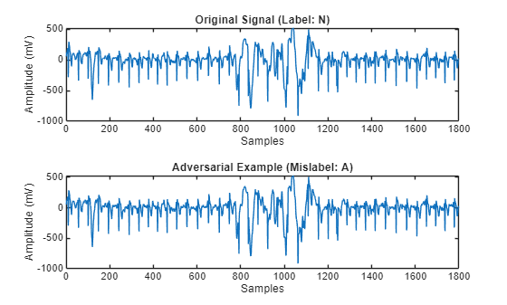

Train Adversarially Robust Network

The adversarial examples are misclassified by the network as mislabel. Use the input batch index iX to find their expected true label.

correctedLabel = TTrain(iX);

To train a network that is robust to adversarial examples, add the adversarial examples to the training data set.

XTrainAdv = cat(finddim(example,"B"),dlarray(cell2mat(XTrain),"BTC"),example);
TTrainAdv = cat(1,TTrain(:),correctedLabel(:));

Because this data set has more normal signals than atrial fibrillation signals, determine the inverse frequency class weights and create a weighted loss function. For more information, see Train Deep Learning Network for ECG Signal Classification.

classes = unique(TTrain)';
numClasses = numel(classes);

for i=1:numClasses
    classFrequency(i) = sum(TTrainAdv(:) == classes(i));
    classWeights(i) = size(XTrainAdv,finddim(XTrainAdv, "B"))/(numClasses*classFrequency(i));
end

dictionary(classes, classWeights)

ans =

  dictionary (categorical ⟼ double) with 2 entries:

    A ⟼ 4.7898
    N ⟼ 0.5583

lossFcn = @(Y,T) crossentropy(Y,T,classWeights, ...
    NormalizationFactor="all-elements", ...
    WeightsFormat="C")*numClasses;

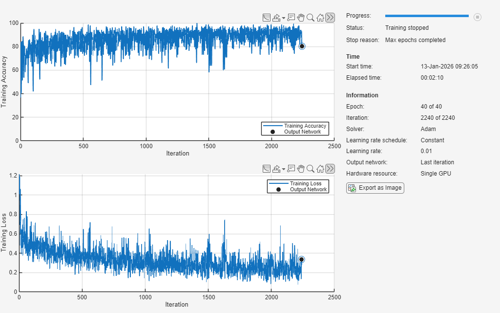
Specify the training options. Choosing among the options requires empirical analysis. To explore different training option configurations by running experiments, you can use the Experiment Manager app. For this example:

Train for 40 epochs using the Adam optimizer with a learn rate of 0.01.
Left-pad the sequences.
Monitor the training progress in a plot and suppress the verbose output.

options = trainingOptions("adam", ...
    MaxEpochs=40, ...
    MiniBatchSize=128, ...
    InitialLearnRate=0.01, ...
    SequencePaddingDirection="left", ...
    Plots="training-progress", ...
    Metrics="accuracy", ...
    Verbose=false, ...
    InputDataFormats="CTB", ...
    Shuffle="every-epoch");

Take the trained network and then continue training it on the adversarial examples by using the trainnet function. To train the network, set the doTraining flag to true. Otherwise, load a pretrained network.

doTraining = false;

if doTraining
    [netRobust,infoRobust] = trainnet(XTrainAdv,TTrainAdv,net,lossFcn,options);
else
    load("adversariallyTrainedECGNetwork.mat");
show(infoRobust)
end

Test Network on Adversarial Examples

Compute the accuracies of the nonrobust and the robust network on the adversarial example data.

scoresAdv = minibatchpredict(net,example);
YAdv = scores2label(scoresAdv,categories(correctedLabel));
accuracyAdv = mean(YAdv == correctedLabel')

accuracyAdv = 
0

scoresAdvRobust = minibatchpredict(netRobust,example); 
YRobustAdv = scores2label(scoresAdvRobust,categories(correctedLabel)); 
accuracyAdvRobust = mean(YRobustAdv == correctedLabel')

accuracyAdvRobust = 
0.9231

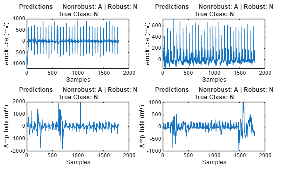
Plot the prediction results for a subset of the adversarial data. For the original network, the accuracy is severely degraded on the adversarial example data. However, the robust network still accurately classifies the signals.

visualizePredictions(example,YAdv,YRobustAdv,correctedLabel)

In the next step of the workflow, test the accuracy of the robust network on the original test data and verify that it satisfies the requirements defined in Define Requirements for ECG Signal Classification Using Deep Learning.

Supporting Functions

The visualizePredictions function generates a visualization of four signals along with their predicted classes for the nonrobust and the robust network and the true class.

function visualizePredictions(adversarialInputs,nonrobustPrediction,robustPrediction,trueLabel)

figure

numImages = 4;
tiledlayout('flow',Padding="compact",TileSpacing="compact");

% Select random images from the data.
indices = randperm(size(adversarialInputs,2),numImages);

adversarialInputs = extractdata(adversarialInputs);
adversarialInputs = adversarialInputs(:,indices,:);
nonrobustPrediction = nonrobustPrediction(indices);
robustPrediction = robustPrediction(indices);
trueLabel = trueLabel(indices);

% Plot images with the predicted label.
for i = 1:numImages
    nexttile
    plot(squeeze(adversarialInputs(:, i, :)))

    predictionText = sprintf("Predictions — Nonrobust: %s | Robust: %s", ...
        string(nonrobustPrediction(i)), string(robustPrediction(i)));

    trueClassText = sprintf("True Class: %s",string(trueLabel(i)));

    title({predictionText,trueClassText});

    xlabel("Samples");
    ylabel("Amplitude (mV)");
end
end

Improve Adversarial Robustness of Deep Learning Network for ECG Signal Classification

Generate Adversarial Examples

Train Adversarially Robust Network

Test Network on Adversarial Examples

Supporting Functions

See Also

Topics