findAdversarialExamples
Find adversarial examples for MATLAB, ONNX, and PyTorch classification networks
Since R2026a
Syntax
Description
Add-On Required: This feature requires the AI Verification Library for Deep Learning Toolbox add-on.
dlnetwork adversarial examples
[
also returns index vectors example,mislabel,iX,iE] = findAdversarialExamples(net,XLower,XUpper,label)iX and iE. You can
find adversarial examples for several sets of input bounds and labels at once. However,
the findAdversarialExamples function does not always find an
adversarial example. If the generated example is not misclassified as expected, then the
function does not return it. Therefore, the batch dimension of
example can be smaller than the batch dimensions of
XLower, XUpper, and
label. To find out which example corresponds to which set of inputs,
use the index vectors iX and iE to index into
the example and input batches, respectively.
___ = findAdversarialExamples(___,AdversarialLabel=adversarialLabel)
creates targeted adversarial examples that the network incorrectly classifies as
adversarialLabel instead of label.
___ = findAdversarialExamples(___,
specifies additional options using one or more name-value arguments.Name=Value)
ONNX and PyTorch network adversarial examples
This syntax requires the Deep Learning Toolbox Interface for alpha-beta-CROWN Verifier add-on.
[
creates untargeted adversarial examples example,mislabel] = findAdversarialExamples(modelfile,XLower,XUpper,label,numClasses)example between
XLower and XUpper from the pretrained
ONNX™ or PyTorch® network in modelfile. Specify the expected correct
label using the label argument and the number of classes in the
network with the numClasses argument. The function also returns the
actual predicted label mislabel
[
also returns index vectors example,mislabel,iX,iE] = findAdversarialExamples(modelfile,XLower,XUpper,label,numClasses)iX and iE. You can
find adversarial examples for several sets of input bounds and labels at once. However,
the findAdversarialExamples function does not always find an
adversarial example. If the created example is not misclassified as expected, then the
function does not return it. Therefore, the batch dimension of
example can be smaller than the batch dimensions of
XLower, XUpper, and
label. To find out which example corresponds to which set of inputs,
use the index vectors iX and iE to index into
the example and input batches, respectively.
___ = findAdversarialExamples(___,
specifies additional options using one or more name-value arguments.Name=Value)
Examples
Load a pretrained network. This network has been trained to classify images of digits.
rng(1)
load("digitsClassificationConvolutionNet.mat","net")
classNames = categorical(0:9);
Load the test dataset, then randomly select a subset of samples to use for generating adversarial examples.
[XTest,TTest] = digitTest4DArrayData;

numInputs = 10;
testIdx = randi(numel(TTest),numInputs);
imgs = XTest(:,:,:,testIdx);
labels = TTest(testIdx,:);
Prepare the data by converting it to a dlarray object.
X = dlarray(single(imgs),"SSCB");Find the labels predicted by the network.
scores = predict(net,X);
YTest = scores2label(scores,classNames);
In this example, the values of the pixels are between 0 and 1, so specify a maximum perturbation size of 0.1. Clip the lower and upper bounds so that they remain within the range of the input data.
perturbationSize = 0.1;

XLower = max(X-perturbationSize,0);
XUpper = min(X+perturbationSize,1);
Use the findAdversarialExamples function to find adversarial examples.
[examples,mislabels,iX] = findAdversarialExamples(net,XLower,XUpper,labels);
For the first adversarial example, view the original image and the adversarial example side-by-side. The adversarial example is misclassified even though the adversarial image appears very similar to the original image.
adversarialExampleIndex = 1;
inputIndex = iX(adversarialExampleIndex);

figure
tiledlayout(1,2);

nexttile(1);
imshow(imgs(:,:,:,inputIndex));
title({"Original Image (Class: " + string(labels(inputIndex)) + ")", ...
    "Predicted Class: " + string(YTest(inputIndex))});

nexttile(2)
imshow(extractdata(examples(:,:,:,adversarialExampleIndex)));
title({"Adversarial Example (Class: " + string(labels(inputIndex)) + ")", ...
    "Predicted Class: " + string(mislabels(1))});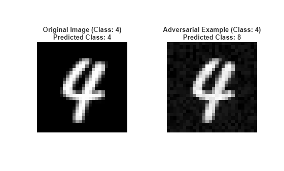
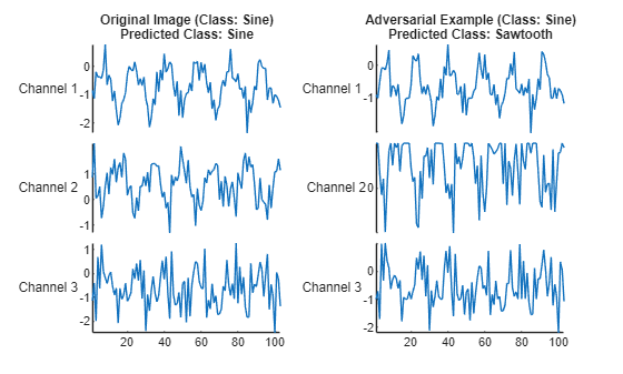
Load a pretrained network. This network has been trained to classify waveforms into one of four classes: sawtooth, sine, square, or triangle.
rng("default")
load("trainedWaveformClassificationNetwork.mat","net")
Load a test input.
load("WaveformData");
classNames = unique(labels)
classNames = 4×1 categorical
Sawtooth
Sine
Square
Triangle
numChannels = size(data{1},2);
testIdx = 1;
input = data{testIdx};
label = labels(testIdx)
label = categorical
Sine
Prepare the input by converting it to a dlarray object.
X = dlarray(single(input),"TC");Find the class predicted by the network.
score = predict(net,X);
YTest = scores2label(score,classNames)
YTest = categorical
     Sine
Find adversarial examples. As this data has values in the range [-1,1], specify a maximum perturbation size of 0.3.
perturbationSize = 0.3;

XLower = max(X-perturbationSize,-1);
XUpper = min(X+perturbationSize,1);
To specify additional options, create an adversarialOptions object. Set the step size to 0.1 and the number of iterations to 50.
options = adversarialOptions("bim",StepSize=0.1,NumIterations=50)options =
AdversarialOptionsBIM with properties:
StepSize: 0.1000
NumIterations: 50
MiniBatchSize: 128
ExecutionEnvironment: 'auto'
Verbose: 0
Use the findAdversarialExamples function to find an adversarial example for the test input. If no example is found, the function returns []. Find an adversarial example that misclassifies the input as "Sawtooth".
[example,mislabel] = findAdversarialExamples(net,XLower,XUpper,label, ...
    Algorithm=options,AdversarialLabel=categorical("Sawtooth",string(classNames)));
View the original input and the adversarial example side-by-side.
figure
tiledlayout(1,2);

nexttile(1);
stackedplot(input,DisplayLabels="Channel "+string(1:numChannels))
title({"Original Image (Class: " + string(label) + ")", ...
    "Predicted Class: " + string(YTest)});

nexttile(2)
    stackedplot(extractdata(squeeze(example))',DisplayLabels="Channel "+string(1:numChannels));
title({"Adversarial Example (Class: " + string(label) + ")", ...
    "Predicted Class: " + string(mislabel)});
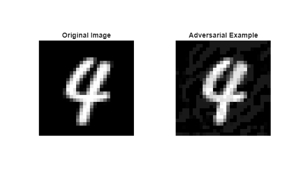
Load a pretrained classification network. This network is a PyTorch® model that has been trained to predict the class label of images of handwritten digits.
rng(1)
modelfile = "digitsClassificationConvolutionNet.pt";
numClasses = 10;
Load the test dataset, then randomly select a subset of samples to use for generating adversarial examples.
[XTest,TTest] = digitTest4DArrayData;
numInputs = 10;
testIdx = randi(numel(TTest),numInputs);
X = XTest(:,:,:,testIdx);
labels = TTest(testIdx,:);
In this example, the values of the pixels are between 0 and 1, so specify a maximum perturbation size of 0.1. Clip the lower and upper bounds so that they remain within the range of the input data.
perturbationSize = 0.1;
XLower = max(X-perturbationSize,0);
XUpper = min(X+perturbationSize,1);
Use the findAdversarialExamples function to generate adversarial examples.
[examples,mislabels,iX] = findAdversarialExamples(modelfile,XLower,XUpper,labels,numClasses, ...
    Algorithm="bim", ...
    InputDataPermutation=[4 3 1 2]);
For the first adversarial example, view the original image and the adversarial example side-by-side.
adversarialExampleIndex = 1;
inputIndex = iX(adversarialExampleIndex);

figure
tiledlayout(1,2);
nexttile(1);
imshow(X(:,:,:,inputIndex));
title("Original Image");

nexttile(2)
imshow(extractdata(examples(:,:,:,adversarialExampleIndex)));
title("Adversarial Example");
Load a pretrained network. This network has been trained to classify natural RGB images.
rng("default")
[net,classNames] = imagePretrainedNetwork;
inputSize = net.Layers(1).InputSize(1:2);
Load a test image and resize it to the expected network input size. This is an image of a golden retriever.
img = imread("sherlock.jpg");
img = imresize(img,inputSize);
X = dlarray(single(img),"SSCB");

label = categorical("golden retriever",classNames);
Find the label predicted by the network.
score = predict(net,X);
YTest = scores2label(score,classNames)
YTest = categorical
     golden retriever
This image has values in the range [0 255]. Generate lower and upper bounds with a maximum perturbation size of ∓10. Ensure that the values do not go below 0 or above 255.
perturbationSize = 10;

XLower = max(X-perturbationSize,0);
XUpper = min(X+perturbationSize,255);
The default step size is suitable for inputs with values between [0,1]. As this input has values with a maximum of 255, create an adversarial options object with a step size of 1 and number of iterations set to 2.
options = adversarialOptions("bim",StepSize=1,NumIterations=2);
[example,mislabel] = findAdversarialExamples(net,XLower,XUpper,label,Algorithm=options);
View the original image and the adversarial example side-by-side. The adversarial example is misclassified even though the adversarial image appears very similar to the original image.
figure
tiledlayout(1,2);

nexttile(1);
imshow(img);
title({"Original Image (Class: " + string(label) + ")", ...
    "Predicted Class: " + string(YTest)});
nexttile(2)
imshow(uint8(extractdata(example)));
title({"Adversarial Example", "Predicted Class: " + string(mislabel)});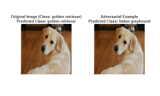
Input Arguments
Name-Value Arguments
Output Arguments
More About
Algorithms
References
[1] Goodfellow, Ian J., Jonathon Shlens, and Christian Szegedy. “Explaining and Harnessing Adversarial Examples.” Preprint, submitted March 20, 2015. https://arxiv.org/abs/1412.6572.
Version History
Introduced in R2026a