使用物理信息神经网络求解 ODE

此示例说明如何训练物理信息神经网络 (PINN) 来预测常微分方程 (ODE) 的解。

并非所有微分方程都有闭式解。为了找到这些类型的方程的近似解，有许多传统的数值算法可供使用。物理信息神经网络 (PINN) [1] 是一种将物理定律融入其结构体和训练过程的神经网络。您可以训练一个神经网络，输出定义物理系统的 ODE 的解。这种方法具有诸多优势，包括以封闭解析形式提供可微分的近似解 [2]。

此示例说明如何完成以下操作：

生成 $x \in [0, 2]$ 范围内的训练数据。
定义一个神经网络，该网络以 $x$ 为输入，并返回在 $x$ 处计算的 ODE $\dot{y} = - 2 xy$ 的近似解作为输出。
使用自定义损失函数训练网络。
将网络预测结果与解析解进行比较。

ODE 和损失函数

在此示例中，您将求解 ODE

$\dot{y} = - 2 xy,$

初始条件为 $y (0) = 1$ 。此 ODE 的解析解为

$y (x) = e^{- x^{2}} .$

定义一个自定义损失函数，该函数对不满足 ODE 和初始条件的偏差进行罚分。在此示例中，损失函数是 ODE 损失和初始条件损失的加权和：

$L_{θ} (x) = ‖ {y_{}^{˙}}_{θ} + 2 x y_{θ} ‖^{2} + k ‖ y_{θ} (0) - 1 ‖^{2}$

$θ$ 是网络参数， $k$ 是常量系数， $y_{θ}$ 是网络预测的解， $\dot{y_{θ}}$ 是使用自动微分计算的预测解的导数。 $‖ \dot{y_{θ}} + 2 {xy}_{θ} ‖^{2}$ 项是 ODE 损失，它量化了预测解与满足 ODE 定义的偏差程度。 $‖ y_{θ} (0) - 1 ‖^{2}$ 项是初始条件损失，它量化了预测解与满足初始条件的偏差程度。

生成输入数据并定义网络

在 $x \in [0, 2]$ 范围内生成 10,000 个训练数据点。

x = linspace(0,2,10000)';

定义用于求解 ODE 的网络。由于输入是实数 $x \in R$ ，因此指定输入大小为 1。

inputSize = 1;
layers = [
    featureInputLayer(inputSize,Normalization="none")
    fullyConnectedLayer(10)
    sigmoidLayer
    fullyConnectedLayer(1)
    sigmoidLayer];

基于层数组创建一个 dlnetwork 对象。

net = dlnetwork(layers)

net = 
  dlnetwork with properties:

         Layers: [5×1 nnet.cnn.layer.Layer]
    Connections: [4×2 table]
     Learnables: [4×3 table]
          State: [0×3 table]
     InputNames: {'input'}
    OutputNames: {'layer_2'}
    Initialized: 1

  View summary with summary.

定义模型损失函数

创建在示例的模型损失函数部分列出的函数 modelLoss，该函数以神经网络、小批量输入数据和与初始条件损失关联的系数为输入。此函数返回损失以及该损失关于神经网络中可学习参数的梯度。

指定训练选项

使用 100 的小批量大小进行 15 轮训练。

numEpochs = 15;
miniBatchSize = 100;

指定 SGDM 优化的选项。指定学习率为 0.5、学习率下降因子为 0.5、学习率下降周期为 5、动量为 0.9。

initialLearnRate = 0.5;
learnRateDropFactor = 0.5;
learnRateDropPeriod = 5;
momentum = 0.9;

指定损失函数中初始条件项的系数为 7。此系数指定了初始条件对损失的相对贡献。调整此参数可以帮助训练更快地收敛。

icCoeff = 7;

训练模型

要在训练期间使用小批量数据，请执行以下操作：

基于训练数据创建一个 arrayDatastore 对象。
创建一个以 arrayDatastore 对象为输入的 minibatchqueue 对象，指定小批量大小以丢弃部分小批量，并且训练数据的格式为 "BC"（批量、通道）。

默认情况下，minibatchqueue 对象将数据转换为基础类型为 single 的 dlarray 对象。如果 GPU 可用，该对象还会将每个输出都转换为一个 gpuArray。使用 GPU 需要 Parallel Computing Toolbox™ 和支持的 GPU 设备。有关受支持设备的信息，请参阅GPU 计算要求 (Parallel Computing Toolbox)。

ads = arrayDatastore(x,IterationDimension=1);
mbq = minibatchqueue(ads, ...
    MiniBatchSize=miniBatchSize, ...
    PartialMiniBatch="discard", ...
    MiniBatchFormat="BC");

初始化 SGDM 求解器的速度参数。

velocity = [];

计算训练进度监视器的总迭代次数。

numObservationsTrain = numel(x);
numIterationsPerEpoch = floor(numObservationsTrain / miniBatchSize);
numIterations = numEpochs * numIterationsPerEpoch;

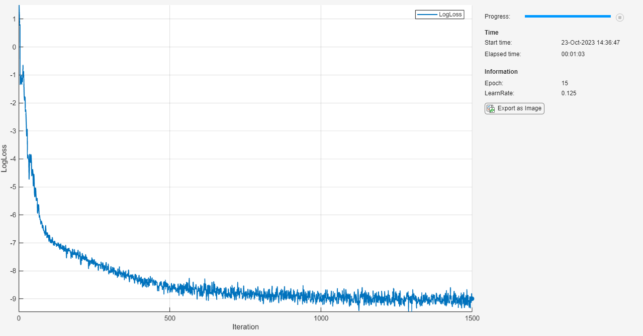
初始化 TrainingProgressMonitor 对象。由于计时器在您创建监视器对象时启动，请确保您创建的对象靠近训练循环。

monitor = trainingProgressMonitor( ...
    Metrics="LogLoss", ...
    Info=["Epoch" "LearnRate"], ...
    XLabel="Iteration");

使用自定义训练循环来训练网络。对于每轮训练，对数据进行乱序处理，并遍历小批量数据。对于每个小批量：

使用 dlfeval 和 modelLoss 函数计算模型损失和梯度。
使用 sgdmupdate 函数更新网络参数。
显示训练进度。
如果 Stop 属性为 true，则停止训练。当您点击“停止”按钮时，TrainingProgressMonitor 对象的 Stop 属性值会更改为 true。

每 learnRateDropPeriod 轮将学习率乘以 learnRateDropFactor。

epoch = 0;
iteration = 0;
learnRate = initialLearnRate;
start = tic;

% Loop over epochs.
while epoch < numEpochs  && ~monitor.Stop
    epoch = epoch + 1;

    % Shuffle data.
    mbq.shuffle

    % Loop over mini-batches.
    while hasdata(mbq) && ~monitor.Stop

        iteration = iteration + 1;

        % Read mini-batch of data.
        X = next(mbq);

        % Evaluate the model gradients and loss using dlfeval and the modelLoss function.
        [loss,gradients] = dlfeval(@modelLoss, net, X, icCoeff);

        % Update network parameters using the SGDM optimizer.
        [net,velocity] = sgdmupdate(net,gradients,velocity,learnRate,momentum);

        % Update the training progress monitor.
        recordMetrics(monitor,iteration,LogLoss=log(loss));
        updateInfo(monitor,Epoch=epoch,LearnRate=learnRate);
        monitor.Progress = 100 * iteration/numIterations;

    end
    
    % Reduce the learning rate.
    if mod(epoch,learnRateDropPeriod)==0
        learnRate = learnRate*learnRateDropFactor;
    end
end

测试模型

通过将网络预测结果与解析解进行比较来测试网络的准确度。

生成 $x \in [0, 4]$ 范围内的测试数据，以查看网络是否能够在训练范围 $x \in [0, 2]$ 之外进行外插。

xTest = linspace(0,4,1000)';

使用 minibatchpredict 函数进行预测。默认情况下，minibatchpredict 函数使用 GPU（如果有）。使用 GPU 需要 Parallel Computing Toolbox™ 许可证和受支持的 GPU 设备。有关受支持设备的信息，请参阅GPU 计算要求 (Parallel Computing Toolbox)。否则，该函数使用 CPU。要指定执行环境，请使用 ExecutionEnvironment 选项。

yModel = minibatchpredict(net,xTest);

计算解析解。

yAnalytic = exp(-xTest.^2);

通过以对数刻度绘制解析解和模型预测来对它们进行比较。

figure;
plot(xTest,yAnalytic,"-")
hold on
plot(xTest,yModel,"--")
legend("Analytic","Model")
xlabel("x")
ylabel("y (log scale)")
set(gca,YScale="log")

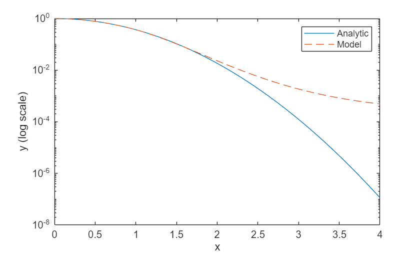
模型在训练范围 $x \in [0, 2]$ 内准确地逼近解析解，并在 $x \in (2, 4]$ 范围内进行外插，但准确度较低。

计算训练范围 $x \in [0, 2]$ 内的均方相对误差。

yModelTrain = yModel(1:500);
yAnalyticTrain = yAnalytic(1:500);

errorTrain = mean(((yModelTrain-yAnalyticTrain)./yAnalyticTrain).^2)

errorTrain = single

0.0029

计算外插范围 $x \in (2, 4]$ 内的均方相对误差。

yModelExtra = yModel(501:1000);
yAnalyticExtra = yAnalytic(501:1000);

errorExtra = mean(((yModelExtra-yAnalyticExtra)./yAnalyticExtra).^2)

errorExtra = single

6.9634e+05

请注意，外插范围内的均方相对误差高于训练范围内的均方相对误差。

模型损失函数

modelLoss 函数以 dlnetwork 对象 net、小批量输入数据 X 和与初始条件损失关联的系数 icCoeff 为输入。此函数返回损失关于 net 中可学习参数的梯度以及相应损失。损失定义为 ODE 损失和初始条件损失的加权和。计算此损失需要二阶导数。要能够进行二阶自动微分，请使用函数 dlgradient 并将 EnableHigherDerivatives 名称值参量设置为 true。

function [loss,gradients] = modelLoss(net, X, icCoeff)
y = forward(net,X);

% Evaluate the gradient of y with respect to x. 
% Since another derivative will be taken, set EnableHigherDerivatives to true.
dy = dlgradient(sum(y,"all"),X,EnableHigherDerivatives=true);

% Define ODE loss.
eq = dy + 2*y.*X;

% Define initial condition loss.
ic = forward(net,dlarray(0,"CB")) - 1;

% Specify the loss as a weighted sum of the ODE loss and the initial condition loss.
loss = mean(eq.^2,"all") + icCoeff * ic.^2;

% Evaluate model gradients.
gradients = dlgradient(loss, net.Learnables);

end

参考资料

Maziar Raissi, Paris Perdikaris, and George Em Karniadakis, Physics Informed Deep Learning (Part I):Data-driven Solutions of Nonlinear Partial Differential Equations https://arxiv.org/abs/1711.10561
Lagaris, I. E., A. Likas, and D. I. Fotiadis.“Artificial Neural Networks for Solving Ordinary and Partial Differential Equations.”IEEE Transactions on Neural Networks 9, no. 5 (September 1998):987–1000. https://doi.org/10.1109/72.712178.

另请参阅

dlarray | dlfeval | dlgradient