使用傅里叶神经算子求解 PDE

此示例说明如何训练傅里叶神经算子 (FNO) 神经网络来输出偏微分方程 (PDE) 的解。

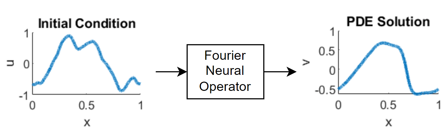
神经算子 [1] 是一种能够在函数空间之间进行映射的神经网络。例如，当给定系统的初始条件时，它可以学习输出 PDE 的解。傅里叶神经算子 (FNO) [2] 是一种能够利用傅里叶变换更高效地学习这些映射的神经算子。具体而言，对于空间域中的输入函数 $f$ ，神经网络中的各层学习变换 $F$ ，使得 $F (f) = f_{}^{ˆ}$ ，其中 $f_{}^{ˆ}$ 是 $f$ 的傅里叶变换。然后 FNO 可以在频域中进行运算。使用神经网络来预测 PDE 的解，可能比数值求解更快。

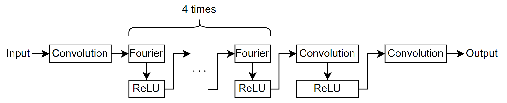
下图说明了数据在 FNO 中的流动过程。

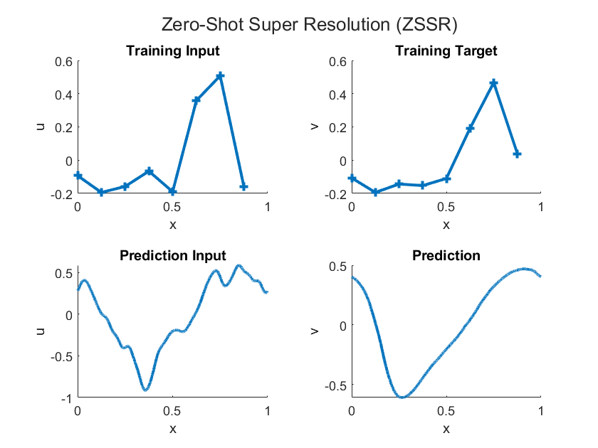
Diagram of data flowing through FNO. The input is a function labeled "Initial Condition". The output is a function labeled "PDE Solution".

由于 FNO 学习的是函数空间之间的映射，您可以在比训练数据分辨率更高的条件下计算输出函数。该功能被称为零样本超分辨率 (ZSSR)。也就是说，ZSSR 能够在无需额外高分辨率样本的情况下，将输入和输出数据的分辨率提升到原始训练数据之上。下图说明了用于预测的低分辨率训练数据与高分辨率输入输出之间的差异。

Plots showing low resolution and high resolution inputs and outputs. The low-resolution functions are composed of a small number of straight lines between points. The high-resolution functions are smooth curves.

此示例训练一个 FNO 来输出一维伯格斯方程的解。

加载训练数据

加载一维伯格斯方程的数据。

伯格斯方程是一中 PDE，它在应用数学的多个领域（如流体力学、非线性声学、气体动力学和交通流）中都有出现。该 PDE 为：

$\frac{\partial u}{\partial t} + u \frac{\partial u}{\partial x} = \frac{1}{R e} \frac{\partial^{2} u}{\partial x^{2}}, x \in (0, 1), t \in (0, 1),$

其中 $R e$ 是雷诺数。初始条件为：

$u (x, 0) = u_{0} (x), x \in (0, 1)$

该方程在整个空间域上施加周期性边界条件，将初始条件 $u_{0}$ 映射到以下时间处的解： $t = 1 : u_{0} ⟼ u (x, 1)$ 。

从 burgers_data_R10.mat 加载一维伯格斯方程的数据，其中包含初始速度 $u_{0}$ 和伯格斯方程的解 $u (x, 1)$ 。

dataFile = "burgers_data_R10.mat";
if ~exist(dataFile,"file")
    location = "https://ssd.mathworks.com/supportfiles/nnet/data/burgers1d/burgers_data_R10.mat";
    websave(dataFile,location); 
end

data = load(dataFile,"a","u");
u0 = data.a;
u1 = data.u;

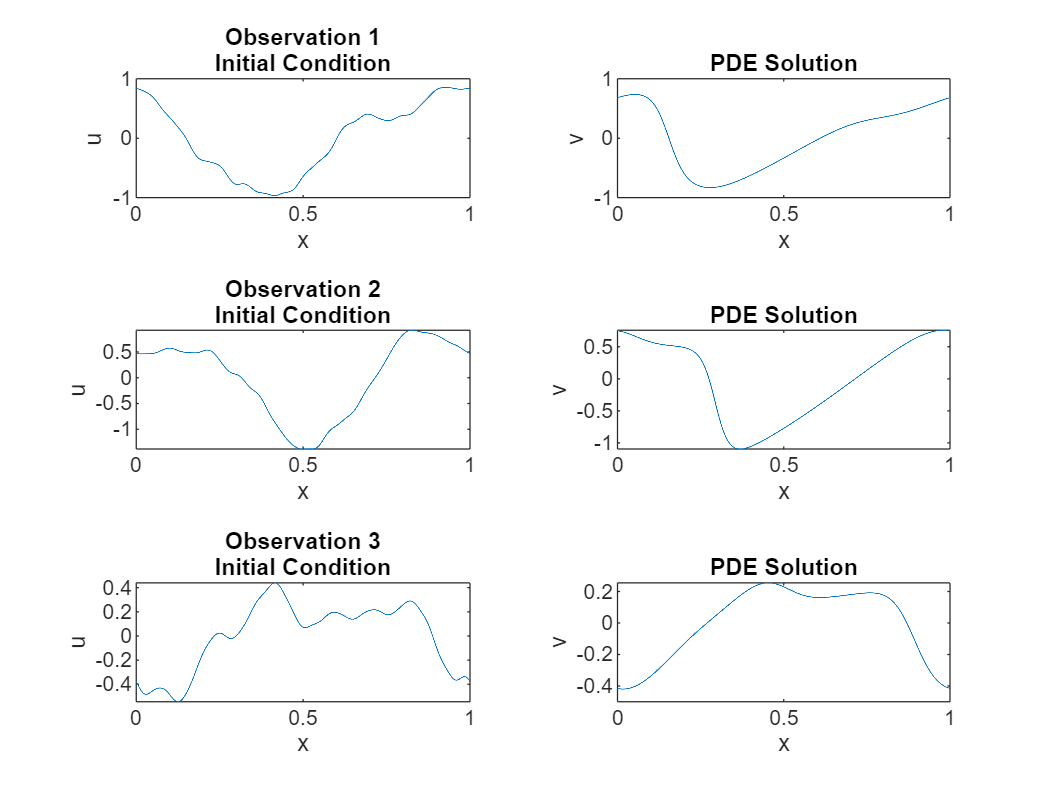
查看其中一些训练数据。

numPlots = 3;
gridSize = size(u0,2);
figure
tiledlayout(numPlots,2)
for i = 1:numPlots
    nexttile
    plot(linspace(0,1,gridSize),u0(i,:));
    title("Observation " + i + newline + "Initial Condition")
    xlabel("x")
    ylabel("u")

    nexttile
    plot(linspace(0,1,gridSize),u1(i,:));
    title("PDE Solution")
    xlabel("x")
    ylabel("v")
end

准备训练数据

使用 trainingPartitions 函数来拆分训练数据和测试数据，此函数作为支持文件包含在此示例中。要访问此函数，请以实时脚本形式打开此示例。将 80% 的数据用于训练，10% 用于验证，其余 10% 用于测试。

numObservations = size(u0,1);
[idxTrain,idxValidation,idxTest] = trainingPartitions(numObservations,[0.8 0.1 0.1]);
U0Train = u0(idxTrain,:);
U1Train = u1(idxTrain,:);

U0Validation = u0(idxValidation,:);
U1Validation = u1(idxValidation,:);
U0Test = u0(idxTest,:);

为减少 FNO 中的处理量，对训练数据和验证数据进行下采样，使其网格大小为 1024。

gridSizeDownsampled = 1024;
downsampleFactor = floor(gridSize./gridSizeDownsampled);

U0Train = U0Train(:,1:downsampleFactor:end);
U1Train = U1Train(:,1:downsampleFactor:end);
U0Validation = U0Validation(:,1:downsampleFactor:end);
U1Validation = U1Validation(:,1:downsampleFactor:end);

FNO 要求输入数据有一个对应于空间坐标（网格）的通道。创建该网格并将其与输入数据串联。

xMin = 0;
xMax = 1;
xGrid = linspace(xMin,xMax,gridSizeDownsampled);

xGridTrain = repmat(xGrid, [numel(idxTrain) 1]);
xGridValidation = repmat(xGrid, [numel(idxValidation) 1]);

U0Train = cat(3,U0Train,xGridTrain);
U0Validation = cat(3,U0Validation,xGridValidation);

查看训练集和验证集的大小。第一个维度、第二个维度和第三个维度分别是批量维度、空间维度和通道维度。

size(U0Train)

ans = 1×3

    1638    1024    2

size(U0Validation)

ans = 1×3

    204    1024    2

定义神经网络架构

定义神经网络架构。该网络由多个傅里叶层和卷积层组成。

定义傅里叶层

定义一个函数，用于创建在频域中运算的网络层。

该层通过应用卷积和频谱卷积处理输入，并对输出求和。下图说明了该层的架构。

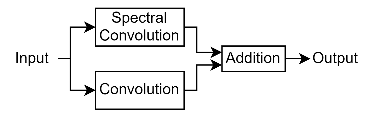
Diagram showing FNO layer architecture. The input is connected to both a spectral convolution layer and a convolution layer. The outputs of the two convolution layers are connected to an addition layer. The output of the FNO layer is the output of the addition layer.

频谱卷积层在频域中应用矩阵乘法，由于它允许网络学习复杂的空间依赖关系，因此对于求解 PDE 特别有用。为了应用频谱卷积运算，傅里叶层使用 spectralConvolution1dLayer 对象。

function layer = fourierLayer(numModes,spatialWidth,args)

arguments
    numModes
    spatialWidth
    args.Name = ""
end
name = args.Name;

net = dlnetwork;

layers = [
    identityLayer(Name="in")
    spectralConvolution1dLayer(numModes,spatialWidth,Name="specConv")
    additionLayer(2,Name="add")];

net = addLayers(net,layers);

layer = convolution1dLayer(1,spatialWidth,Name="fc");
net = addLayers(net,layer);

net = connectLayers(net,"in","fc");
net = connectLayers(net,"fc","add/in2");

layer = networkLayer(net,Name=name);

end

创建神经网络

定义神经网络架构。此示例中的网络由多个按顺序连接的傅里叶 ReLU 模块组成。

Diagram of the neural network of layers connected in series. From left to right, there is the input, convolution, four fourier-ReLU blocks, convolution, ReLU, convolution, and output.

指定以下选项：

对于傅里叶层，指定 16 个模式，空间宽度为 16。
使用大小为 [NaN spatialWidth 2]、格式为 "BSC"（批量、空间、通道）的输入层，其中 spatialWidth 是傅里叶层的空间宽度。
为卷积 ReLU 模块指定 128 个 1×1 滤波器。
对于最后的卷积层，指定一个 1×1 滤波器。

numModes = 16;
spatialWidth = 64; 

layers = [
    inputLayer([NaN spatialWidth 2],"BSC");
    convolution1dLayer(1,spatialWidth,Name="fc0")
    fourierLayer(numModes,spatialWidth,Name="fourier1");
    reluLayer
    fourierLayer(numModes,spatialWidth,Name="fourier2")
    reluLayer
    fourierLayer(numModes,spatialWidth,Name="fourier3")
    reluLayer
    fourierLayer(numModes,spatialWidth,Name="fourier4")
    reluLayer
    convolution1dLayer(1,128)
    reluLayer
    convolution1dLayer(1,1)];

训练选项

指定训练选项。在选项中进行选择需要经验分析。要通过运行试验探索不同训练选项配置，您可以使用Experiment Manager。

使用 SGDM 求解器进行训练。
使用分段学习率调度进行训练，初始学习率为 0.001，下降因子为 0.5。
使用 20 的小批量大小进行 40 轮训练。
每轮训练都会打乱数据。
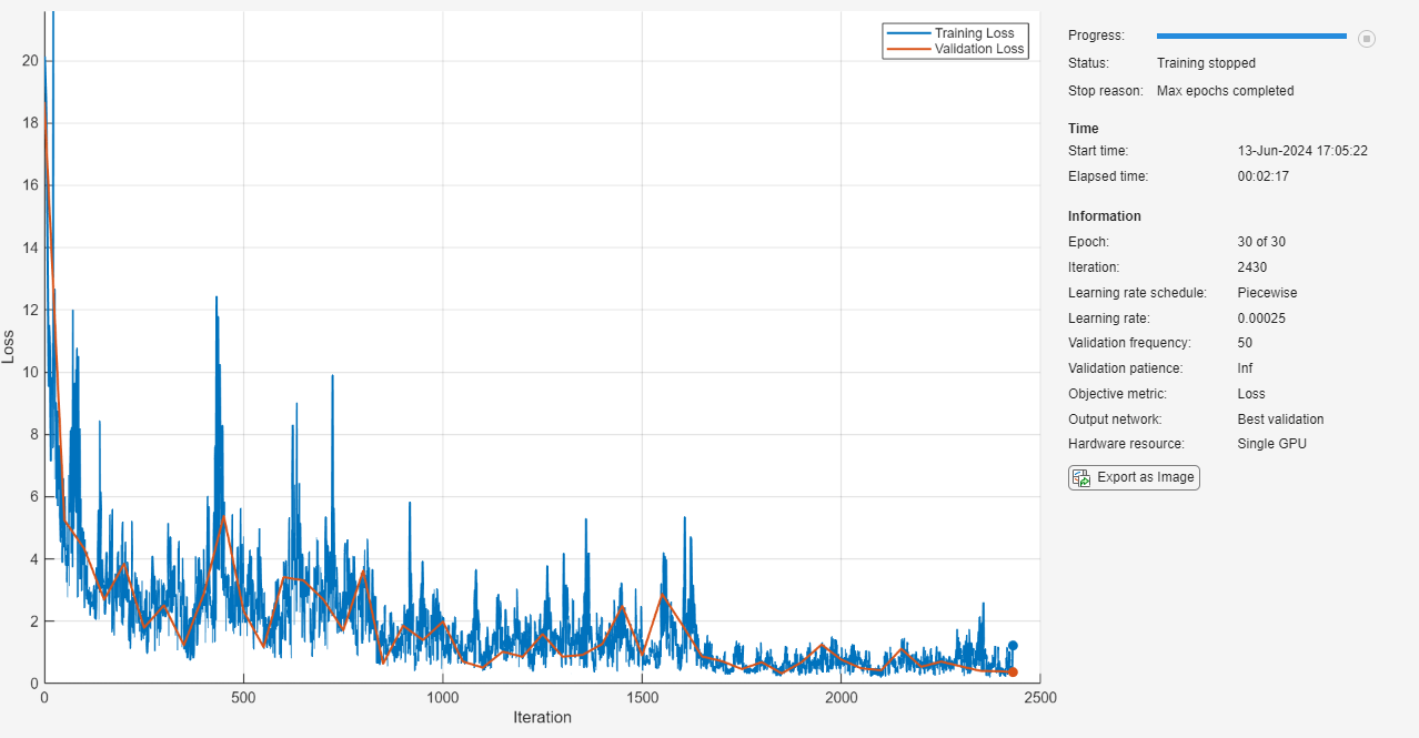
由于输入数据的维度对应于批量维度、空间维度和通道维度，因此将输入数据格式指定为 "BSC"。
在图中监控训练进度。
指定验证数据，并每 100 次迭代验证一次网络。
禁用详尽输出。

schedule = piecewiseLearnRate(DropFactor=0.5);

options = trainingOptions("sgdm", ...
    InitialLearnRate=1e-3, ...
    LearnRateSchedule=schedule, ...
    MaxEpochs=40, ...
    MiniBatchSize=20, ...
    Shuffle="every-epoch", ...
    InputDataFormats="BSC", ...
    Plots="training-progress", ...
    ValidationData={U0Validation,U1Validation}, ...
    ValidationFrequency=100, ...
    Verbose=false);

定义相对 $L_{2}$ 损失函数

创建函数 relativeL2Loss，该函数以预测值和目标作为输入，并返回相对 $L_{2}$ 损失。相对 $L_{2}$ 损失函数是 $L_{2}$ 损失函数的一种变体，它通过使用预测值与目标之间差值的欧几里德范数，再除以目标的欧几里德范数来考虑尺度因素：

$R e l a t i v e L 2 (Y, T) = \sum_{n = 1}^{N} \frac{‖ T_{n} - Y_{n} ‖_{2}}{‖ T_{n} ‖_{2}}$

其中：

$Y$ 表示预测值。
$T$ 表示目标。
$N$ 表示观测值数量。

function loss = relativeL2Loss(Y,T)

Y = stripdims(Y,"BSC");
T = stripdims(T,"BSC");

p = vecnorm(T-Y,2,2);
q = vecnorm(T,2,2);

loss = sum(p./q, 1);

end

训练网络

使用 trainnet 函数训练神经网络。使用自定义损失函数 relativeL2Loss。默认情况下，trainnet 函数使用 GPU（如果有）。使用 GPU 需要 Parallel Computing Toolbox™ 许可证和受支持的 GPU 设备。有关受支持设备的信息，请参阅GPU 计算要求 (Parallel Computing Toolbox)。否则，该函数使用 CPU。要手动选择执行环境，请使用 ExecutionEnvironment 训练选项。

net = trainnet(U0Train,U1Train,layers,@relativeL2Loss,options);

测试网络

通过将模型对保留测试集的预测值与真实标签进行比较，并计算均方根误差 (RMSE)，来测试模型的预测性能。

对测试数据进行下采样，并使用与训练数据相同的步骤串联网格。

xGridTest = repmat(xGrid, [numel(idxTest) 1]);

U0Test = U0Test(:,1:downsampleFactor:end);
U0Test = cat(3,U0Test,xGridTest);

U1Test = u1(idxTest,:);
U1Test = U1Test(:,1:downsampleFactor:end);

使用 testnet 函数测试神经网络。默认情况下，testnet 函数使用 GPU（如果有）。否则，该函数使用 CPU。要手动选择执行环境，请使用 testnet 函数的 ExecutionEnvironment 参量。

rmseTest = testnet(net,U0Test,U1Test,"rmse")

rmseTest = 
0.0092

为评估 ZSSR 的准确度，使用未下采样的测试数据来测试网络。

xGridZSSR = linspace(xMin,xMax,gridSize);
xGridTestZSSR = repmat(xGridZSSR, [numel(idxTest) 1]);

U0TestZSSR = u0(idxTest,:);
U0TestZSSR = cat(3,U0TestZSSR,xGridTestZSSR);
U1TestZSSR = u1(idxTest,:);

rmseTestZSSR = testnet(net,U0TestZSSR,U1TestZSSR,"rmse")

rmseTestZSSR = 
0.0354

使用新数据进行预测

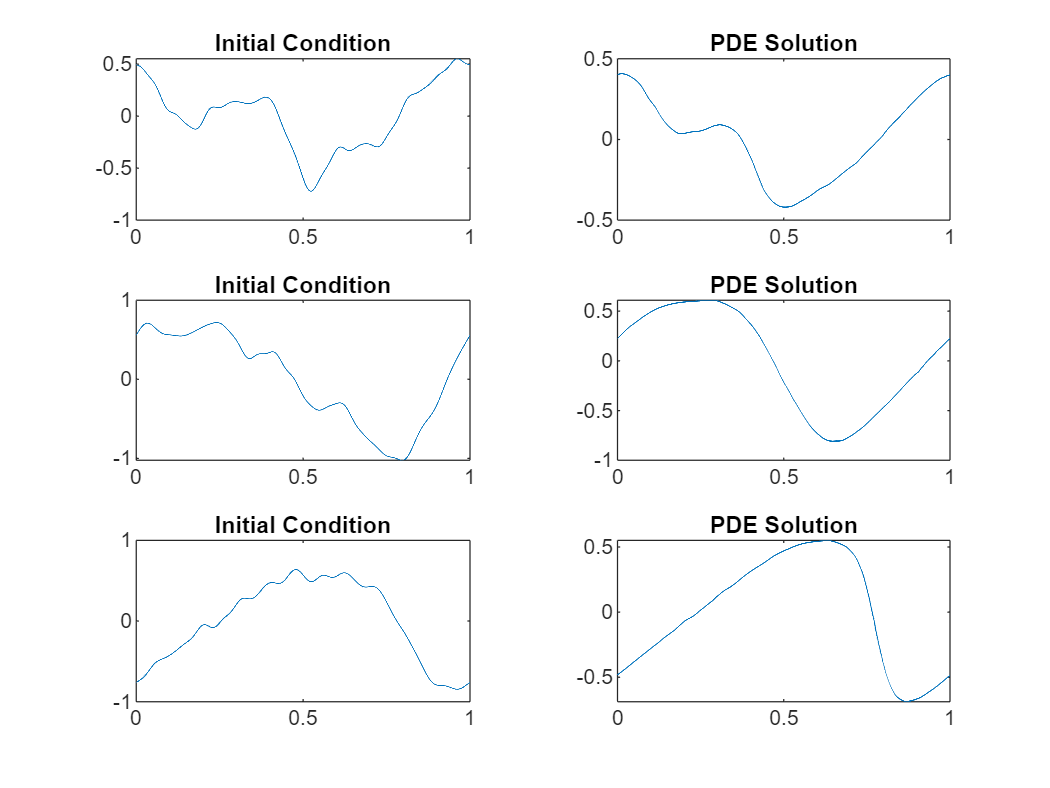
加载新数据。出于示例目的，使用前三个测试观测值。

dataNew = u0(idxTest(1:3),:);
numObservationsNew = size(dataNew,1);

计算网格大小并将其与数据串联。

gridSizeNew = size(dataNew,2);
xGridNew = linspace(xMin,xMax,gridSizeNew);
xGridNew = repmat(xGridNew, [size(dataNew,1) 1]);
U0New = cat(3,dataNew,xGridNew);

使用 minibatchpredict 函数进行预测。默认情况下，minibatchpredict 函数使用 GPU（如果有）。否则，该函数使用 CPU。要手动选择执行环境，请使用 ExecutionEnvironment 选项。

Y = minibatchpredict(net,U0New);

在图中可视化预测。

figure
tiledlayout(numObservationsNew,2)
for i = 1:numObservationsNew
    nexttile
    plot(xGridNew(i,:),dataNew(i,:))
    title("Initial Condition")

    nexttile
    plot(xGridNew(i,:),Y(i,:))
    title("PDE Solution")
end

参考资料

Li, Zongyi, Nikola Kovachki, Kamyar Azizzadenesheli, Burigede Liu, Kaushik Bhattacharya, Andrew Stuart, and Anima Anandkumar.“Neural Operator:Graph Kernel Network for Partial Differential Equations.” arXiv, March 6, 2020. http://arxiv.org/abs/2003.03485.
Li, Zongyi, Nikola Kovachki, Kamyar Azizzadenesheli, Burigede Liu, Kaushik Bhattacharya, Andrew Stuart, and Anima Anandkumar.“Fourier Neural Operator for Parametric Partial Differential Equations,” 2020. https://openreview.net/forum?id=c8P9NQVtmnO.

另请参阅

spectralConvolution1dLayer | trainingOptions | trainnet | dlnetwork