基于小波散射和深度学习的口述数字识别
此示例说明如何使用机器学习和深度学习方法对语音数字进行分类。在此示例中,您将使用小波时间散射配合支持向量机 (SVM) 和长短期记忆 (LSTM) 网络执行分类。您还可以应用贝叶斯优化来确定合适的超参数,以提高 LSTM 网络的准确度。此外,该示例说明了一种使用深度卷积神经网络 (CNN) 和 Mel 频谱图的方法。
数据
请下载免费的口述数字数据集 (FSDD) [1]。FSDD 包含四个说话者分别朗读英文数字 0 至 9 的 2000 个录音。两个说话者以美式英语为母语,另外两个说话者不以英语为母语且分别带有比利时法语和德语口音。数据以 8000 Hz 的频率采样。
downloadFolder = matlab.internal.examples.downloadSupportFile("audio","FSDD.zip");
dataFolder = tempdir;
unzip(downloadFolder,dataFolder)
dataset = fullfile(dataFolder,"FSDD");
使用 audioDatastore (Audio Toolbox) 管理数据访问,并确保将录音随机分为训练集和测试集。创建一个指向该数据集的 audioDatastore。
ads = audioDatastore(dataset,IncludeSubfolders=true);
辅助函数 helpergenLabels 基于 FSDD 文件创建标签分类数组。附录中列出了 helpergenLabels 的源代码。列出各类和每个类中的示例数量。
ads.Labels = helpergenLabels(ads);
summary(ads.Labels)
2000×1 categorical

     0                200
     1                200
     2                200
     3                200
     4                200
     5                200
     6                200
     7                200
     8                200
     9                200
     <undefined>        0
FSDD 数据集由 10 个平衡类组成,每个平衡类有 200 个录音。FSDD 的录音时间长度不等。FSDD 不是特别大,因此通读 FSDD 文件并构造信号长度直方图。
LenSig = zeros(numel(ads.Files),1);
nr = 1;
while hasdata(ads)
    digit = read(ads);
    LenSig(nr) = numel(digit);
    nr = nr+1;
end
reset(ads)
histogram(LenSig)
grid on
xlabel("Signal Length (Samples)")
ylabel("Frequency")
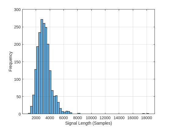
直方图显示录音长度呈正偏态分布。对于分类,此示例使用 8192 个采样点这一常见信号长度,这是保守值,可确保截断较长的录音不会切断语音内容。如果信号长度大于 8192 个采样点(1.024 秒),录音将被截断为 8192 个采样点。如果信号长度小于 8192 个采样点,将以对称方式用零对信号进行前置和后置填充,使其达到 8192 个采样点的长度。
小波时间散射
使用 waveletScattering (Wavelet Toolbox) 以 0.22 秒的不变性尺度创建小波时间散射框架。在此示例中,通过对所有时间采样点的散射变换求平均值来创建特征向量。要使每个时间窗的散射系数数量足以求平均值,请将 OversamplingFactor 设置为 2,以使每条路径的散射系数数量相对于临界下采样值增加为原来的四倍。
sf = waveletScattering(SignalLength=8192,InvarianceScale=0.22, ...
    SamplingFrequency=8000,OversamplingFactor=2);
将 FSDD 分成训练集和测试集。将 80% 的数据分配给训练集,将 20% 保留给测试集。训练数据用于基于散射变换训练分类器。测试数据用于验证模型。
rng("default")
ads = shuffle(ads);
[adsTrain,adsTest] = splitEachLabel(ads,0.8);
countEachLabel(adsTrain)ans=10×2 table
0 160
1 160
2 160
3 160
4 160
5 160
6 160
7 160
8 160
9 160
countEachLabel(adsTest)
ans=10×2 table
    0    40
    1    40
    2    40
    3    40
    4    40
    5    40
    6    40
    7    40
    8    40
    9    40
辅助函数 helperReadSPData 将数据截断或填充为 8192 的长度,并将每个录音按其最大值进行归一化。附录中列出了 helperReadSPData 的源代码。创建一个 8192×1600 矩阵,其中每列是一个语音数字录音。
Xtrain = [];
scatds_Train = transform(adsTrain,@(x)helperReadSPData(x));
while hasdata(scatds_Train)
    smat = read(scatds_Train);
    Xtrain = cat(2,Xtrain,smat);
end
对测试集重复该过程。生成的矩阵为 8192×400。
Xtest = [];
scatds_Test = transform(adsTest,@(x)helperReadSPData(x));
while hasdata(scatds_Test)
    smat = read(scatds_Test);
    Xtest = cat(2,Xtest,smat);
end
对训练集和测试集应用小波散射变换。
Strain = sf.featureMatrix(Xtrain);
Stest = sf.featureMatrix(Xtest);
获取训练集和测试集的散射特征均值。排除零阶散射系数。
TrainFeatures = Strain(2:end,:,:);
TrainFeatures = squeeze(mean(TrainFeatures,2))';
TestFeatures = Stest(2:end,:,:);
TestFeatures = squeeze(mean(TestFeatures,2))';
SVM 分类器
现在数据已简化为针对每个记录有一个特征向量,下一步是使用这些特征对录音进行分类。用二次多项式核创建一个 SVM 学习器模板。对训练数据进行 SVM 拟合。
template = templateSVM(...
    KernelFunction="polynomial", ...
    PolynomialOrder=2, ...
    KernelScale="auto", ...
    BoxConstraint=1, ...
    Standardize=true);
classificationSVM = fitcecoc( ...
    TrainFeatures, ...
    adsTrain.Labels, ...
    Learners=template, ...
    Coding="onevsone", ...
    ClassNames=categorical({'0'; '1'; '2'; '3'; '4'; '5'; '6'; '7'; '8'; '9'}));
使用 k 折交叉验证来基于训练数据预测模型的泛化准确度。将训练集分成五个组。
partitionedModel = crossval(classificationSVM,KFold=5);
[validationPredictions, validationScores] = kfoldPredict(partitionedModel);
validationAccuracy = (1 - kfoldLoss(partitionedModel,LossFun="ClassifError"))*100
validationAccuracy = 96.9375
估计的泛化准确度约为 97%。使用经过训练的 SVM 预测测试集中的口述数字类。
predLabels = predict(classificationSVM,TestFeatures);
testAccuracy = sum(predLabels==adsTest.Labels)/numel(predLabels)*100 %#ok<NASGU>
testAccuracy = 98
用混淆图总结模型基于测试集的预测效果。使用列汇总和行汇总显示每个类的准确率和召回率。混淆图底部的表显示每个类的精确率值。混淆图右侧的表显示召回值。
figure(Units="normalized",Position=[0.2 0.2 0.5 0.5])
ccscat = confusionchart(adsTest.Labels,predLabels);
ccscat.Title = "Wavelet Scattering Classification";
ccscat.ColumnSummary = "column-normalized";
ccscat.RowSummary = "row-normalized";

使用散射变换配合 SVM 分类器对测试集中的口述数字进行分类,准确度达到 98%(即错误率为 2%)。
长短期记忆 (LSTM) 网络
LSTM 网络是一种循环神经网络 (RNN)。RNN 是专门用于处理序列或时序数据(如语音数据)的神经网络。由于小波散射系数是序列,因此它们可以用作 LSTM 的输入。通过使用散射特征而不是原始数据,您可以减少网络需要学习的变异性。
修改用于 LSTM 网络的训练和测试散射特征。排除零阶散射系数,并将特征转换为元胞数组。
TrainFeatures = Strain(2:end,:,:);
TrainFeatures = squeeze(num2cell(TrainFeatures,[1 2]));
TestFeatures = Stest(2:end,:,:);
TestFeatures = squeeze(num2cell(TestFeatures, [1 2]));
构造一个包含 256 个隐藏层的简单 LSTM 网络。
[inputSize, ~] = size(TrainFeatures{1});
YTrain = adsTrain.Labels;

numHiddenUnits = 256;
numClasses = numel(unique(YTrain));

layers = [ ...
    sequenceInputLayer(inputSize)
    lstmLayer(numHiddenUnits,OutputMode="last")
    fullyConnectedLayer(numClasses)
    softmaxLayer];
设置超参数。使用 Adam 优化和小批量大小为 50。将最大训练轮数设置为 300。使用 1e-4 作为学习率。如果您不想使用绘图跟踪进度,可以关闭训练进度绘图。默认情况下,训练使用 GPU(如果有)。否则,将使用 CPU。有关详细信息,请参阅trainingOptions。
maxEpochs = 300;
miniBatchSize = 50;

options = trainingOptions("adam", ...
    InitialLearnRate=1e-4,...
    MaxEpochs=maxEpochs, ...
    MiniBatchSize=miniBatchSize, ...
    SequenceLength="shortest", ...
    Shuffle="every-epoch",...
    Verbose=false, ...
    Plots="training-progress", ...
    Metrics="accuracy", ...
    InputDataFormats="CTB");
训练网络。
net = trainnet(TrainFeatures,YTrain,layers,"crossentropy",options);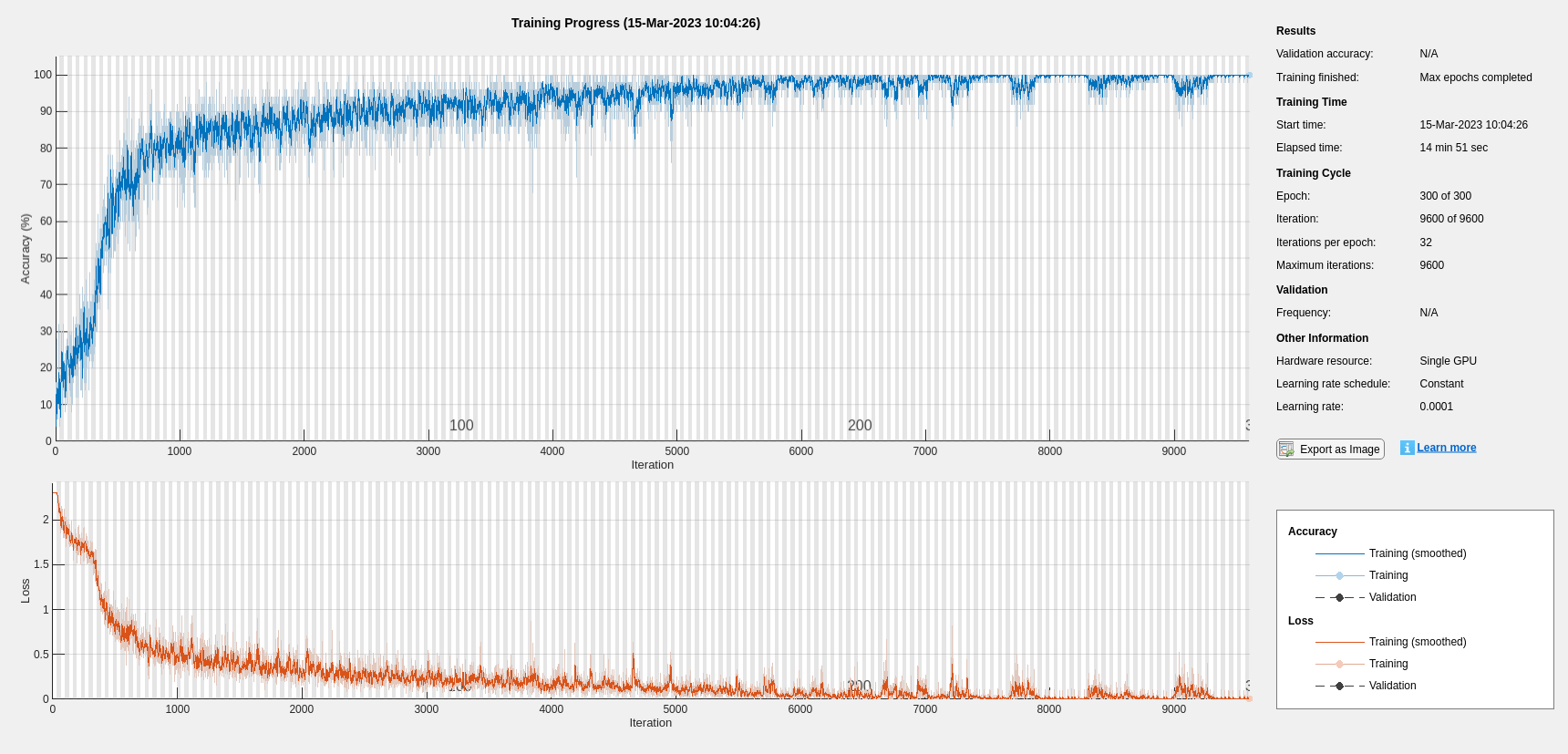
scores = minibatchpredict(net,TestFeatures,InputDataFormats="CTB");
classNames = categories(ads.Labels);
predLabels = scores2label(scores,classNames);
testAccuracy = sum(predLabels==adsTest.Labels)/numel(predLabels)*100 %#ok<NASGU>
testAccuracy =
93.7500
贝叶斯优化
确定合适的超参数设置通常是训练深度网络最困难的部分之一。您可以使用贝叶斯优化来帮助解决这一难题。在此示例中,您将使用贝叶斯方法优化隐藏层的数量和初始学习率。创建一个新目录来存储 MAT 文件,其中包含有关超参数设置和网络的信息以及相应的错误率。
YTrain = adsTrain.Labels;
YTest = adsTest.Labels;

if ~exist("results/",'dir')
    mkdir results
end
初始化要优化的变量及其值范围。由于隐藏层的数量必须为整数,请将 'type' 设置为 'integer'。
optVars = [
    optimizableVariable(InitialLearnRate=[1e-5, 1e-2],Transform="log")
    optimizableVariable(NumHiddenUnits=[100, 1000],Type="integer")
    ];
贝叶斯优化涉及大量计算,可能需要几个小时才能完成。出于此示例的目的,请将 optimizeCondition 设置为 false 以下载并使用预先确定的经过优化的超参数设置。如果您将 optimizeCondition 设置为 true,将使用贝叶斯优化最小化目标函数 helperBayesOptLSTM。附录中列出的目标函数是给定特定超参数设置时网络的错误率。加载的设置是针对目标函数最小值 0.02(2% 错误率)。
ObjFcn = helperBayesOptLSTM(TrainFeatures,YTrain,TestFeatures,YTest);

optimizeCondition = false;
if optimizeCondition
    BayesObject = bayesopt(ObjFcn,optVars, ...
            MaxObjectiveEvaluations=15, ...
            IsObjectiveDeterministic=false, ...
            UseParallel=false); %#ok<UNRCH>
else
    url = "http://ssd.mathworks.com/supportfiles/audio/SpokenDigitRecognition.zip";
    downloadNetFolder = tempdir;
    netFolder = fullfile(downloadNetFolder,"SpokenDigitRecognition");
    if ~exist(netFolder,"dir")
        disp("Downloading pretrained network (1 file - 12 MB) ...")
        unzip(url,downloadNetFolder)
    end
    file = load(fullfile(netFolder,"0.02.mat"));
end
如果执行贝叶斯优化,将生成类似以下的图形,以跟踪目标函数值以及对应的超参数值和迭代次数。您可以增加贝叶斯优化迭代的次数,以确保达到目标函数的全局最小值。
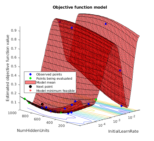

使用隐藏单元数量和初始学习率的优化值,重新训练网络。
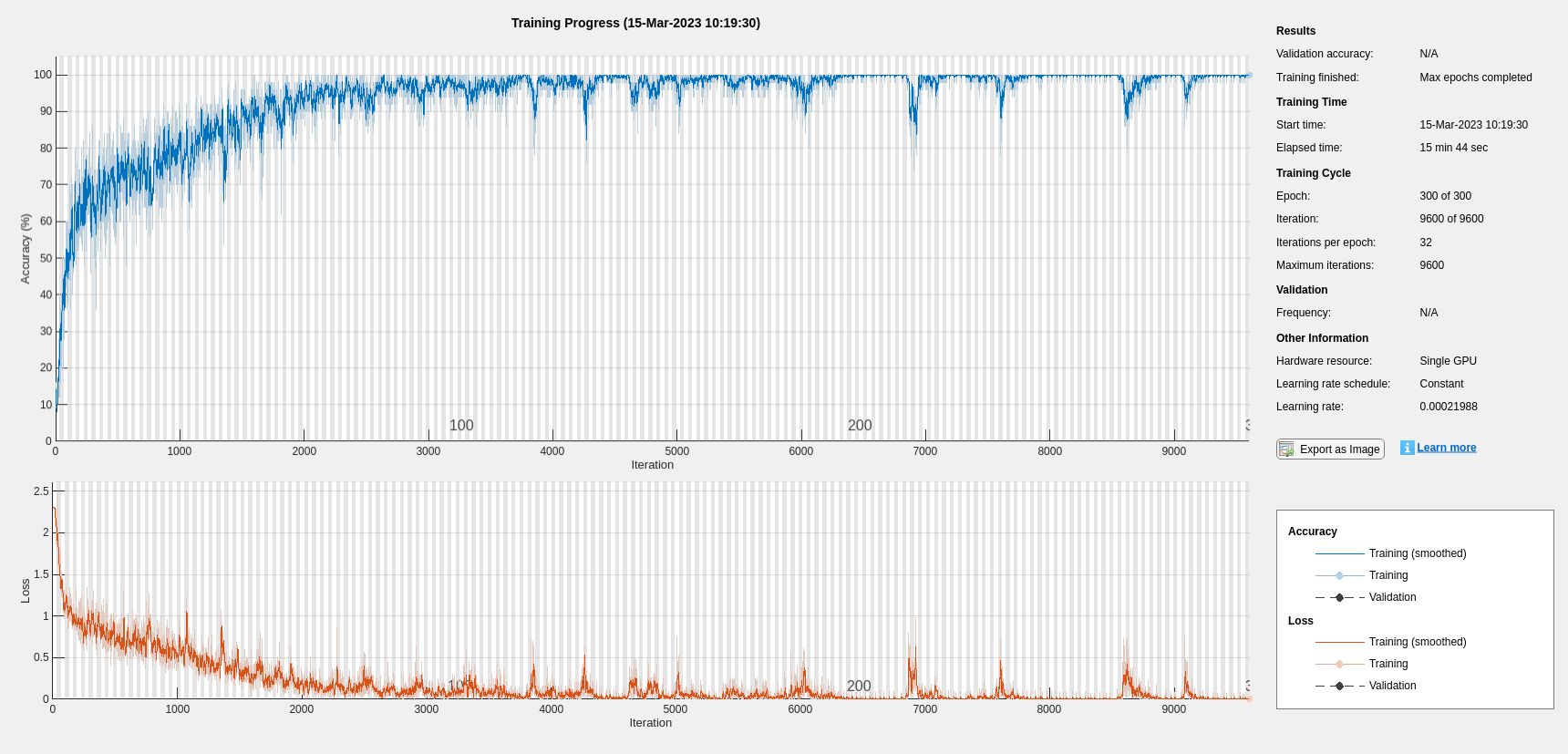
bestNumHiddenUnits = 768;
bestInitialLearnRate = 2.198827960269379e-04;


numClasses = numel(unique(YTrain));

layers = [ ...
    sequenceInputLayer(inputSize)
    lstmLayer(bestNumHiddenUnits,OutputMode="last")
    fullyConnectedLayer(numClasses)
    softmaxLayer];

maxEpochs = 300;
miniBatchSize = 50;

options = trainingOptions("adam", ...
    InitialLearnRate=bestInitialLearnRate, ...
    MaxEpochs=maxEpochs, ...
    MiniBatchSize=miniBatchSize, ...
    SequenceLength="shortest", ...
    Shuffle="every-epoch", ...
    Verbose=false, ...
    Plots="training-progress", ...
    Metrics="accuracy", ...
    InputDataFormats="CTB");

net = trainnet(TrainFeatures,YTrain,layers,"crossentropy",options);
scores = minibatchpredict(net,TestFeatures,InputDataFormats="CTB");
classNames = categories(ads.Labels);
predLabels = scores2label(scores,classNames);
testAccuracy = sum(predLabels==adsTest.Labels)/numel(predLabels)*100
testAccuracy = 97.5000
如图所示,使用贝叶斯优化可以得到更高准确度的 LSTM。
使用 Mel 频谱图的深度卷积网络
下面用另一种方法来完成口述数字识别任务,使用基于 Mel 频谱图的深度卷积神经网络 (DCNN) 对 FSDD 数据集进行分类。使用与散射变换中相同的信号截断/填充过程。同样,用每个信号采样点除以最大绝对值来归一化每个录音。为了保持一致,使用与散射变换相同的训练集和测试集。
设置 Mel 频谱图的参数。使用与散射变换中相同的窗(即帧)长度,即 0.22 秒。将窗之间的帧移设置为 10 ms。使用 40 个频带。
segmentDuration = 8192*(1/8000);
frameDuration = 0.22;
hopDuration = 0.01;
numBands = 40;
重置训练和测试数据存储。
reset(adsTrain)
reset(adsTest)
在本示例末尾定义的辅助函数 helperspeechSpectrograms 使用 melSpectrogram (Audio Toolbox) 在标准化录音长度和归一化振幅后获得 Mel 频谱图。使用 Mel 频谱图的对数作为 DCNN 的输入。为了避免对零取对数,请对每个元素加一个小 ε。
epsil = 1e-6;
XTrain = helperspeechSpectrograms(adsTrain,segmentDuration,frameDuration,hopDuration,numBands);
Computing speech spectrograms...
Processed 500 files out of 1600
Processed 1000 files out of 1600
Processed 1500 files out of 1600
...done
XTrain = log10(XTrain + epsil);

XTest = helperspeechSpectrograms(adsTest,segmentDuration,frameDuration,hopDuration,numBands);
Computing speech spectrograms...
...done
XTest = log10(XTest + epsil);

YTrain = adsTrain.Labels;
YTest = adsTest.Labels;
定义 DCNN 架构
构造一个小 DCNN 作为层的数组。使用卷积和批量归一化层,并使用最大池化层对特征图下采样。为了降低网络记住训练数据特定特征的可能性,可为最后一个全连接层的输入添加一个小的丢弃率。
sz = size(XTrain);
specSize = sz(1:2);
imageSize = [specSize 1];

numClasses = numel(categories(YTrain));

dropoutProb = 0.2;
numF = 12;
layers = [
    imageInputLayer(imageSize)

    convolution2dLayer(5,numF,Padding="same")
    batchNormalizationLayer
    reluLayer

    maxPooling2dLayer(3,Stride=2,Padding="same")

    convolution2dLayer(3,2*numF,Padding="same")
    batchNormalizationLayer
    reluLayer

    maxPooling2dLayer(3,Stride=2,Padding="same")

    convolution2dLayer(3,4*numF,Padding="same")
    batchNormalizationLayer
    reluLayer

    maxPooling2dLayer(3,Stride=2,Padding="same")

    convolution2dLayer(3,4*numF,Padding="same")
    batchNormalizationLayer
    reluLayer
    convolution2dLayer(3,4*numF,Padding="same")
    batchNormalizationLayer
    reluLayer

    maxPooling2dLayer(2)

    dropoutLayer(dropoutProb)
    fullyConnectedLayer(numClasses)
    softmaxLayer
    ];
设置用于训练网络的超参数。使用 50 作为小批量大小,1e-4 作为学习率。指定 Adam 优化。您可以通过将执行环境设置为 "gpu" 或 "auto" 在可用的 GPU 上训练网络。有关详细信息,请参阅trainingOptions。
miniBatchSize = 50;
options = trainingOptions("adam", ...
    InitialLearnRate=1e-4, ...
    MaxEpochs=30, ...
    MiniBatchSize=miniBatchSize, ...
    Shuffle="every-epoch", ...
    Plots="training-progress", ...
    Verbose=false, ...
    Metrics="accuracy", ...
    ExecutionEnvironment="auto");
训练网络。
trainedNet = trainnet(XTrain,YTrain,layers,"crossentropy",options);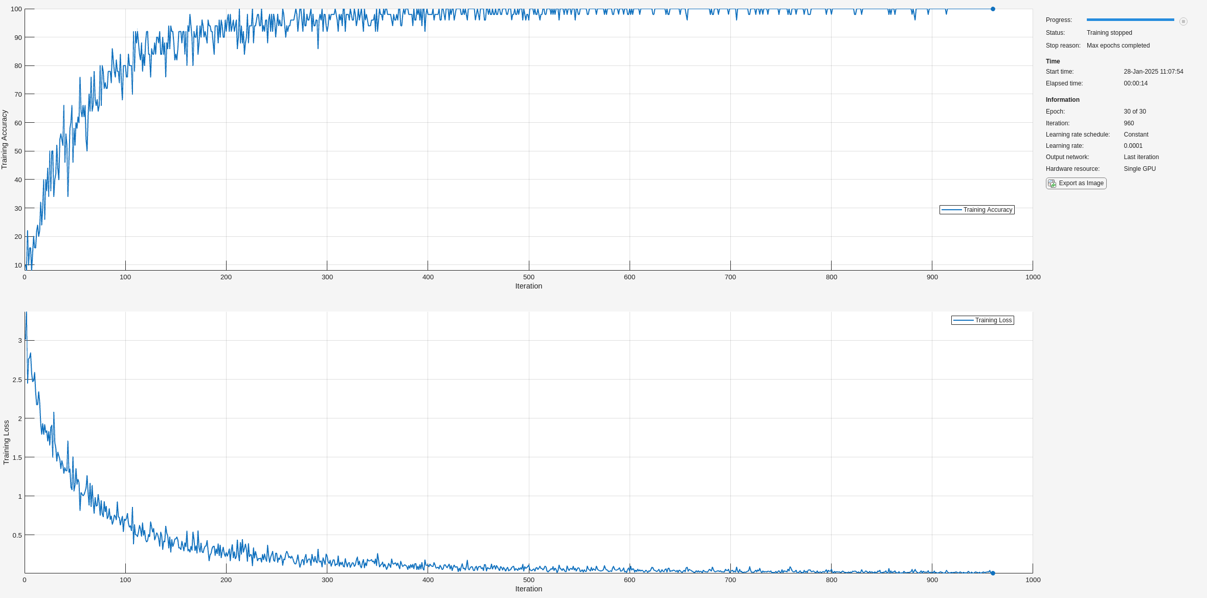
使用经过训练的网络来预测测试集的数字标签。
scores = minibatchpredict(trainedNet,XTest);
classNames = categories(YTrain);
Ypredicted = scores2label(scores,classNames);
cnnAccuracy = sum(Ypredicted==YTest)/numel(YTest)*100
cnnAccuracy =
98.7500
用混淆图总结经过训练的网络基于测试集的性能。使用列汇总和行汇总显示每个类的准确率和召回率。混淆图底部的表显示精确率值。混淆图右侧的表显示召回值。
figure(Units="normalized",Position=[0.2 0.2 0.5 0.5]);
ccDCNN = confusionchart(YTest,Ypredicted);
ccDCNN.Title = "Confusion Chart for DCNN";
ccDCNN.ColumnSummary = "column-normalized";
ccDCNN.RowSummary = "row-normalized";
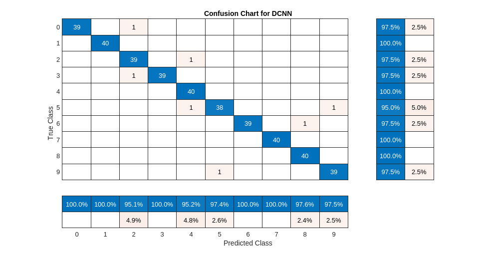
使用 Mel 频谱图作为输入的 DCNN 对测试集中的口述数字进行分类,准确度也约为 98%。
总结
此示例说明如何使用不同的机器和深度学习方法对 FSDD 中的语音数字进行分类。该示例演示了与 SVM 和 LSTM 配对的小波散射。贝叶斯方法用于优化 LSTM 超参数。最后,此示例说明如何将 CNN 和 Mel 频谱图结合使用。
该示例的目标是说明如何使用 MathWorks® 工具以完全不同但互补的方式来解决问题。所有工作流都使用 audioDatastore 来管理来自磁盘的数据流,并确保适当的随机化。
此示例中使用的所有方法在测试集上都表现良好。此示例的目的不是直接比较各种方法。例如,您还可以在 CNN 中使用贝叶斯优化进行超参数选择。适用于此版本 FSDD 之类的小型训练集深度学习的另一个策略是使用数据增强。操作如何影响类并不始终已知,因此数据增强并不始终可行。不过,对于语音,audioDataAugmenter (Audio Toolbox) 能提供可行的数据增强策略。
在使用小波时间散射的情况下,您也可以尝试一些修改。例如,您可以更改变换的不变性尺度,更改每个滤波器组的小波滤波器数量,并尝试不同分类器。
附录:辅助函数
function Labels = helpergenLabels(ads)
% This function is only for use in Wavelet Toolbox examples. It may be
% changed or removed in a future release.
tmp = cell(numel(ads.Files),1);
expression = "[0-9]+_";
for nf = 1:numel(ads.Files)
    idx = regexp(ads.Files{nf},expression);
    tmp{nf} = ads.Files{nf}(idx);
end
Labels = categorical(tmp);
end
function x = helperReadSPData(x)
% This function is only for use Wavelet Toolbox examples. It may change or
% be removed in a future release.

N = numel(x);
if N > 8192
    x = x(1:8192);
elseif N < 8192
    pad = 8192-N;
    prepad = floor(pad/2);
    postpad = ceil(pad/2);
    x = [zeros(prepad,1) ; x ; zeros(postpad,1)];
end
x = x./max(abs(x));

end
function x = helperBayesOptLSTM(X_train, Y_train, X_val, Y_val)
% This function is only for use in the
% "Spoken Digit Recognition with Wavelet Scattering and Deep Learning"
% example. It may change or be removed in a future release.
x = @valErrorFun;

    function [valError,cons, fileName] = valErrorFun(optVars)
        %% LSTM Architecture
        [inputSize,~] = size(X_train{1});
        numClasses = numel(unique(Y_train));

        layers = [ ...
            sequenceInputLayer(inputSize)
            bilstmLayer(optVars.NumHiddenUnits,OutputMode="last") % Using number of hidden layers value from optimizing variable
            fullyConnectedLayer(numClasses)
            softmaxLayer];

        % Plots not displayed during training
        options = trainingOptions("adam", ...
            InitialLearnRate=optVars.InitialLearnRate, ... % Using initial learning rate value from optimizing variable
            MaxEpochs=300, ...
            MiniBatchSize=30, ...
            SequenceLength="shortest", ...
            Shuffle="every-epoch", ...
            Verbose=false, ...
            Metrics="accuracy", ...
            InputDataFormats="CTB");

        %% Train the network
        net = trainnet(X_train, Y_train, layers, "crossentropy", options);
        %% Training accuracy
        scores = minibatchpredict(net,X_val,InputDataFormats="CTB");
        classNames = categories(Y_train);
        X_val_P = scores2label(scores,classNames);
        accuracy_training  = sum(X_val_P == Y_val)./numel(Y_val);
        valError = 1 - accuracy_training;
        %% save results of network and options in a MAT file in the results folder along with the error value
        fileName = fullfile("results", num2str(valError) + ".mat");
        save(fileName,"net","valError","options")
        cons = [];
    end % end for inner function
end % end for outer function
function X = helperspeechSpectrograms(ads,segmentDuration,frameDuration,hopDuration,numBands)
% This function is only for use in the
% "Spoken Digit Recognition with Wavelet Scattering and Deep Learning"
% example. It may change or be removed in a future release.
%
% helperspeechSpectrograms(ads,segmentDuration,frameDuration,hopDuration,numBands)
% computes speech spectrograms for the files in the datastore ads.
% segmentDuration is the total duration of the speech clips (in seconds),
% frameDuration the duration of each spectrogram frame, hopDuration the
% time shift between each spectrogram frame, and numBands the number of
% frequency bands.
disp("Computing speech spectrograms...");

numHops = ceil((segmentDuration - frameDuration)/hopDuration);
numFiles = length(ads.Files);
X = zeros([numBands,numHops,1,numFiles],"single");

for i = 1:numFiles

    [x,info] = read(ads);
    x = normalizeAndResize(x);
    fs = info.SampleRate;
    frameLength = round(frameDuration*fs);
    hopLength = round(hopDuration*fs);

    spec = melSpectrogram(x,fs, ...
        Window=hamming(frameLength,"periodic"), ...
        OverlapLength=frameLength-hopLength, ...
        FFTLength=2048, ...
        NumBands=numBands, ...
        FrequencyRange=[50,4000]);

    % If the spectrogram is less wide than numHops, then put spectrogram in
    % the middle of X.
    w = size(spec,2);
    left = floor((numHops-w)/2)+1;
    ind = left:left+w-1;
    X(:,ind,1,i) = spec;

    if mod(i,500) == 0
        disp("Processed " + i + " files out of " + numFiles)
    end

end

disp("...done");

end

%--------------------------------------------------------------------------
function x = normalizeAndResize(x)
% This function is only for use in the
% "Spoken Digit Recognition with Wavelet Scattering and Deep Learning"
% example. It may change or be removed in a future release.

N = numel(x);
if N > 8192
    x = x(1:8192);
elseif N < 8192
    pad = 8192-N;
    prepad = floor(pad/2);
    postpad = ceil(pad/2);
    x = [zeros(prepad,1) ; x ; zeros(postpad,1)];
end
x = x./max(abs(x));
end
参考资料
[1] Jakobovski.“Jakobovski/Free-Spoken-Digit-Dataset.”GitHub, May 30, 2019. https://github.com/Jakobovski/free-spoken-digit-dataset.
Copyright 2018-2025, The MathWorks, Inc.
另请参阅
trainnet | trainingOptions | dlnetwork