Train Latent ODE Network with Irregularly Sampled Time-Series Data
This example shows how to train a latent ordinary differential equation (ODE) autoencoder with time-series data that is sampled at irregular time intervals.
Most deep learning models for time-series data (for example, recurrent neural networks) require the time-series data to be regularly sampled in order to train. That is, the elements of the sequences must correspond to fixed-width time intervals.
To learn the dynamics of irregularly sampled time-series data, you can use a latent ODE model [1, 2]. A latent ODE model is a variational autoencoder (VAE) [3] that learns the dynamics of time-series data. An autoencoder is a type of model that is trained to replicate its input by transforming the input to a latent space (the encoding step) and reconstructing the input from the latent representation (the decoding step). Training an autoencoder does not require labeled data.
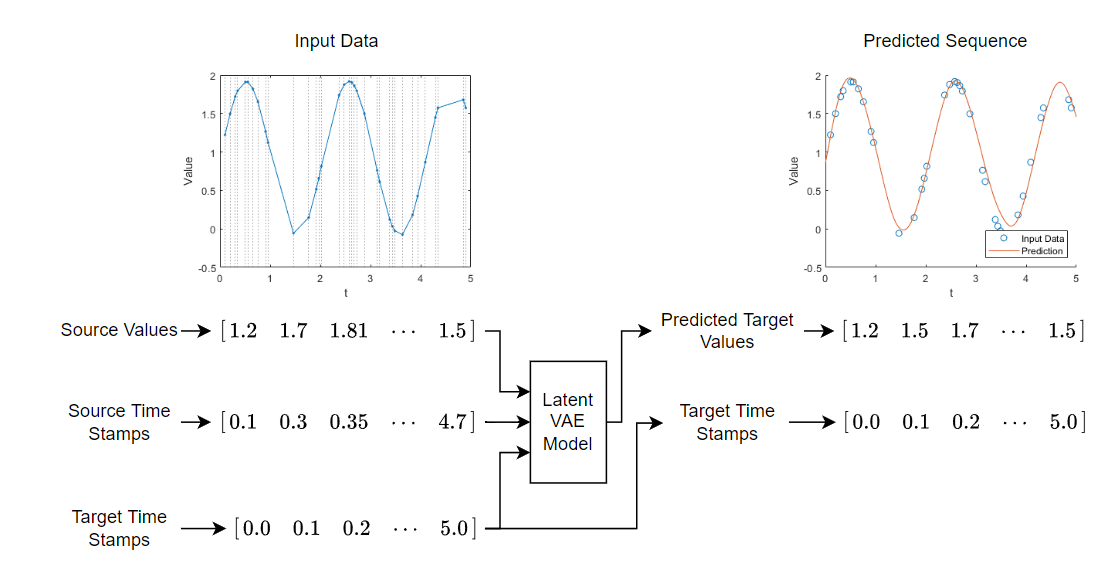
Unlike most autoencoders, a latent ODE model is not trained to replicate its input exactly. Instead, the model learns the dynamics of the input data and you can specify a set of target time stamps, for which the model predicts the corresponding values.
This diagram shows the structure of the model.
Training a latent ODE model takes a long time to run. This example, by default, skips training and loads a pretrained model. To train the model instead, set the doTraining flag to true.
doTraining = false;
Load Data
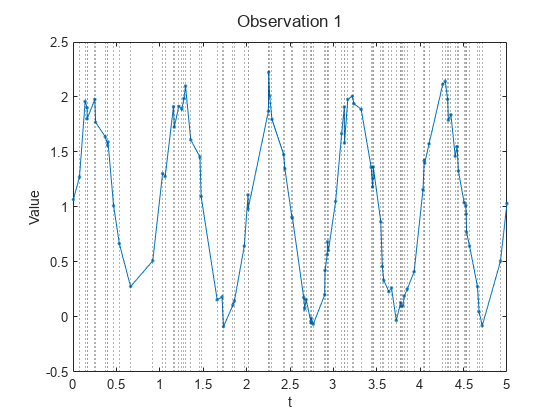
Load the Irregular Sine Waves data set. This data set contains 1000 synthetically generated sine waves with varying frequencies, offsets, and noise. Each sequence uses the same irregularly sampled set of time stamps.
load irregularSineWavesVisualize the first sequence in a plot by looping over the channels. Plot vertical lines that highlight the time stamps. Because the Irregular Sine Waves data set contains only one channel, this code displays a single plot only.
numChannels = size(values,1);

idx = 1;

figure

t = tiledlayout(numChannels,1);
title(t,"Observation " + idx)

for i = 1:numChannels
    nexttile
    plot(tspan,squeeze(values(i,idx,:)),Marker=".");
    xlabel("t")
    ylabel("Value")

    xline(tspan,":")
end
Prepare Data for Training
Split the training and test data using the trainingPartitions function, attached to the example as a supporting file. To access this function, open the example as a live script. Use 80% of the data for training and the remaining 20% for testing.
numObservations = size(values,2);
[idxTrain,idxTest] = trainingPartitions(numObservations,[0.8 0.2]);
sequencesTrain = values(:,idxTrain,:);
sequencesTest = values(:,idxTest,:);
Create datastores that output the training and test data.
dsTrain = arrayDatastore(sequencesTrain,IterationDimension=2);
dsTest = arrayDatastore(sequencesTest,IterationDimension=2);
Initialize Model Learnable Parameters
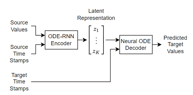
This example trains a VAE, where the encoder uses a recurrent neural network (RNN), known as an ODE-RNN [2] and the decoder is a neural ODE. The encoder maps the sequences to a fixed-length latent representation. This latent representation parameterizes a Gaussian distribution. The model samples from the Gaussian distribution using these encoded parameters and passes the sampled data to the decoder.
This diagram shows the structure of the model.
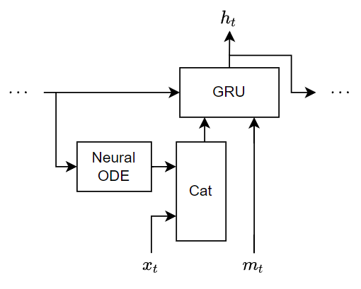
The encoder is an ODE-RNN. It reverses the input sequence so that the last input to the encoder is the first output of the decoder. The ODE-RNN updates the latent representation as it reads each time step of the reversed data using a masked gated recurrent unit (GRU) and an ODE solver. The ODE-RNN concatenates the input data and the hidden state of the GRU operation and advances this output of the GRU operation in time according to the neural ODE. The GRU operation uses the updated state only for time steps specified by the mask.
This diagram shows the structure of the encoder.

This diagram shows the structure of the ODE-RNN when it processes a time step of the data. In this diagram, denotes the value of the time step, denotes the mask value, and is the hidden state output of the GRU operation.
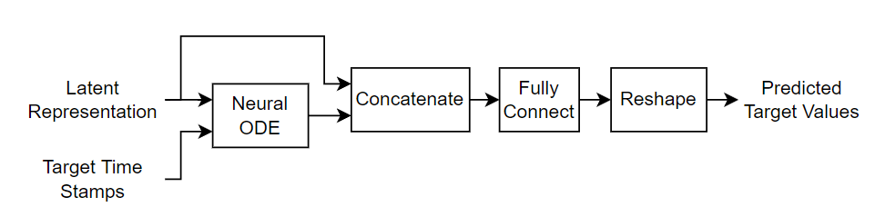
The decoder takes the latent representation and reconstructs the input sequence for the specified target time stamps. The decoder passes the latent representation and the target time stamps to a neural ODE, concatenates the neural ODE output with the latent representation, passes the concatenated data to a fully connect operation, and reshapes the output to match the input sequences.
This diagram shows the structure of the decoder.
To train the model, create a structure that contains the learnable parameters for the latent ODE. Initialize the model learnable parameters using the latentODEParameters function, attached to this example as a supporting file. To access this function, open the example as a live script. The function initializes the learnable parameters for the fully connect and GRU operations by sampling from a narrow-normal distribution (Gaussian distribution with a mean of zero and a standard deviation of 0.01).
Specify the model hyperparameters:
An encoder ODE size of 105
An encoder RNN size of 40
A decoder ODE size of 110
A latent size of 32
encoderODEHiddenSize = 100;
encoderRNNHiddenSize = 40;
decoderODEHiddenSize = 100;
latentSize = 10;

inputSize = numChannels;
parameters = latentODEParameters(inputSize,encoderODEHiddenSize,encoderRNNHiddenSize,latentSize,decoderODEHiddenSize);
Define Model Functions
Define the model functions to use for the deep learning model.
Model Function
The model function, defined in the Model Function section of the example, takes as input the model learnable parameters, the source time stamps and the corresponding sequence values and mask, and the target time stamps. The function returns the predicted values that correspond to the target time stamps.
Encoder Function
The encoder function, defined in the Encoder Function section of the example, takes as input the encoder learnable parameters, the source time stamps, and the corresponding sequence values and mask. The function returns the latent representation.
Decoder Function
The decoder function, defined in the Decoder Function section of the example, takes as input the decoder learnable parameters, the target time stamps, and the latent representation. The function returns the predicted values that correspond to the target time stamps.
Define Model Loss Function
The modelLoss function, defined in the Model Loss Function section of the example, takes as input the model learnable parameters, the time stamps, and the corresponding sequence values and mask. The function returns the model loss and the gradients of the loss with respect to the learnable parameters. The model loss function uses the loss normalized over the number of input observations and samples.
Specify Training Options
Specify these options for training:
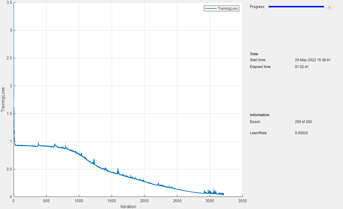
Train for 200 epochs with a mini-batch size of 50.
Train with an initial learning rate of 0.0025.
Decay the learn rate exponentially each iteration with a rate of 0.999 until it reaches 0.00025.
Train using the CPU. Neural ODE models can sometimes train faster on the CPU than on a GPU.
numEpochs = 200;
miniBatchSize = 50;

initialLearnRate = 2.5e-3;
minLearnRate = 2.5e-4;
decayRate = 0.999;

executionEnvironment = "cpu";
Train Model
Train the model in a custom training loop using the loss function modelLoss.
Configure a minibatchqueue object to read out the data.
Preprocess the mini-batches using the
preprocessMiniBatchfunction, listed in the Mini-Batch Preprocessing Function section of the example. This function outputs a mini-batch of sequences with time steps randomly removed and the corresponding mask and target sequence.Specify the mini-batch output formats as
"CBT"(channel, batch, time).Specify the hardware environments of the mini-batch outputs.
numOutputs = 3;
mbqTrain = minibatchqueue(dsTrain,numOutputs,...
    MiniBatchSize=miniBatchSize,...
    MiniBatchFcn=@preprocessMiniBatch,...
    MiniBatchFormat=["CBT" "CBT" "CBT"], ...
    OutputEnvironment=[executionEnvironment executionEnvironment executionEnvironment]);
Initialize the learning rate.
learnRate = initialLearnRate;
Initialize the parameters for the Adam solver.
trailingAvg = [];
trailingAvgSq = [];
To update the progress bar of the training progress monitor, calculate the total number of training iterations.
numObservationsTrain = size(sequencesTrain,2);
numIterationsPerEpoch = ceil(numObservationsTrain/miniBatchSize);
numIterations = numIterationsPerEpoch * numEpochs;
Train the model in a custom training loop. For each epoch, shuffle the training data.
Loop over the mini-batches of training data. For each iteration:
Update the learning rate using exponential decay.
Compute the model loss and gradients using the
dlfevalfunction and themodelLossfunction.Update the learnable parameters using the
adamupdatefunction.Record the training loss in the training progress monitor.
if doTraining

    % Initialize the training progress monitor.
    monitor = trainingProgressMonitor( ...
        Metrics="TrainingLoss", ...
        Info=["LearnRate" "Epoch"]);

    monitor.XLabel = "Iteration";

    % Loop over the epochs.
    epoch = 0;
    iteration = 0;
    while epoch < numEpochs && ~monitor.Stop
        epoch = epoch + 1;

        % Shuffle the training data.
        shuffle(mbqTrain);

        % Loop over the training data.
        while hasdata(mbqTrain) && ~monitor.Stop
            iteration = iteration + 1;

            % Update the learning rate.
            learnRate = max(decayRate*learnRate,minLearnRate);

            % Read a mini-batch of data.
            [X,mask,T] = next(mbqTrain);

            % Calculate the model loss and gradients.
            [loss,gradients] = dlfeval(@modelLoss,parameters,tspan,X,mask,T);

            % Update the learnable parameters.
            [parameters,trailingAvg,trailingAvgSq] = adamupdate(parameters,gradients, ...
                trailingAvg,trailingAvgSq,iteration,learnRate);

            % Update the training progress monitor.
            recordMetrics(monitor,iteration,TrainingLoss=loss);
            updateInfo(monitor,LearnRate=learnRate,Epoch=(epoch+" of "+numEpochs));
            monitor.Progress = 100*(iteration/numIterations);
        end
    end

    % Save the model.
    save("irregularSineWavesParameters.mat","parameters","tspan");
else
    s = load("irregularSineWavesParameters.mat");
    parameters = s.parameters;
    miniBatchSize = s.miniBatchSize;
end
Test Model
Test the model using the test data by creating a mini-batch queue that randomly removes time steps from the sequences and use the trained latent ODE model to predict the removed values.
Create a mini-batch queue that preprocesses the test data using the same steps as the training data.
numOutputs = 2;
mbqTest = minibatchqueue(dsTest,numOutputs,...
    MiniBatchSize=miniBatchSize, ...
    MiniBatchFcn=@preprocessMiniBatch, ...
    MiniBatchFormat=["CBT" "CBT"], ...
    OutputEnvironment=[executionEnvironment executionEnvironment]);
Specify target time stamps to match the original input time stamps.
tspanTarget = tspan;
Make predictions by looping over the mini-batch queue and passing the data through the model.
YTest = [];
while hasdata(mbqTest)
    [X,mask] = next(mbqTest);
    Y = model(parameters,tspan,X,tspanTarget,Mask=mask);
    YTest = cat(2,YTest,Y);
end
Calculate the root-mean-square-error.
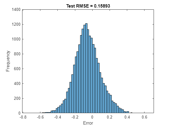
rmse = sqrt(mean((sequencesTest - YTest).^2,"all"))rmse =
1(C) × 1(B) × 1(T) single dlarray
0.1589
Visualize the errors in a histogram.
err = sequencesTest - YTest;
figure
err = extractdata(err);
histogram(err)
xlabel("Error")
ylabel("Frequency")
title("Test RMSE = " + string(rmse))
Predict Using New Data
Reconstruct the test sequences with 1000 equally spaced time stamps between 0 and 5.
Create a mini-batch queue containing the test data.
Preprocess the data using the preprocessMiniBatchPrtedictors function, which creates mini-batches of the sequence data without removing any time steps.
numOutputs = 1;
mbqNew = minibatchqueue(dsTest,numOutputs,...
    MiniBatchSize=miniBatchSize, ...
    MiniBatchFcn=@preprocessMiniBatchPredictors, ...
    MiniBatchFormat="CBT", ...
    OutputEnvironment=executionEnvironment);
Specify 1000 equally spaced time stamps between 0 and 5 as the target time stamps.
tspanTarget = linspace(0,5,1000);
Make predictions by looping over the mini-batch queue.
YNew = modelPredictions(parameters,tspan,mbqNew,tspanTarget);
View the size of the array of predictions.
size(YNew)
ans = 1×3

           1         200        1000
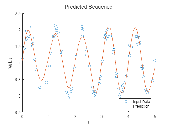
Visualize the first prediction by plotting the inputs in a scatter plot, then plotting the predicted sequences.
Plot the input data.
idx = 1;
X = sequencesTest(:,idx,:);

figure
t = tiledlayout(numChannels,1);
title(t,"Input Sequence")

for i = 1:numChannels
    nexttile
    scatter(tspan,squeeze(X))
    xlabel("t")
    ylabel("Value")
end
Plot the predicted values.
for i = 1:numChannels
    nexttile(i)
    hold on
    plot(tspanTarget,squeeze(YNew(i,idx,:)));
end

title(t,"Predicted Sequence")

legend(["Input Data" "Prediction"],Location="southeast");
Supporting Functions
Model Function
The model function, introduced in the Define Model Functions section of the example, takes as input the model learnable parameters, the source time stamps tspan and the corresponding sequence values and mask, and the target time stamps tspanTarget. The function returns the predicted values Y that correspond to the target time stamps.
This diagram shows the structure of the model function.
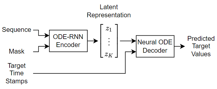
The neural ODE decoder reconstructs the input sequence by sampling from a Gaussian distribution with mean and variance values encoded by its latent representation.
function Y = model(parameters,tspan,X,tspanTarget,args)

arguments
    parameters
    tspan
    X
    tspanTarget
    args.Mask = dlarray(true(size(X)),"CBT")
end

mask = args.Mask;

Z = encoder(parameters.Encoder,tspan,X,Mask=mask);

% Split the latent representation into mean and variance.
latentSize = size(Z,1)/2;
mu = Z(1:latentSize,:);
sigma = abs(Z(latentSize+(1:latentSize),:));

% Take samples of the latent distribution.
epsilon = randn(size(mu),like=X);
Z = epsilon.*sigma + mu;
Z = dlarray(Z,"CB");

% Decode the latent representation.
Y = decoder(parameters.Decoder,tspanTarget,Z);

end
Encoder Function
The encoder function, introduced in the Define Model Functions section of the example, takes as input the encoder learnable parameters, the source time stamps tspan, and the corresponding sequence values and mask. The function outputs the latent representation.
This diagram shows the structure of the encoder.
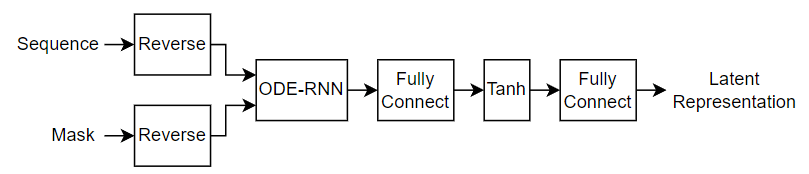
The encoder reverses the input sequence so that the last input to the encoder is the first output of the decoder. The ODE-RNN updates the latent representation as it reads each time step of the reversed data using a masked gated recurrent unit (GRU) and an ODE solver. The ODE-RNN concatenates the input data and the hidden state of the GRU operation and advances this output of the GRU operation in time according to the neural ODE. The GRU operation uses the updated state only for time steps specified by the mask.
This diagram illustrates the structure of the neural ODE-RNN when it processes a time step of the data. In this diagram, denotes the value of the time step, denotes the mask value, and is the hidden state output of the GRU operation. The ODE solver step is a simple fixed-step Euler method for performance.

function Z = encoder(parameters,tspan,X,args)

arguments
    parameters
    tspan
    X
    args.Mask = dlarray(true(size(X)),"CBT")
end

mask = args.Mask;

% Reverse time.
tspan = flip(tspan,2);
X = flip(X,3);
mask = flip(mask,3);

% Initialize the hidden state for the RNN.
hiddenSize = size(parameters.gru.RecurrentWeights,2);
[~,batchSize, sequenceLength] = size(X);
h = zeros(hiddenSize,batchSize,like=X);
h = dlarray(h,"CB");

latentSize = size(parameters.ODE.fc1.Weights,2);

% Solve the ODE-RNN in a loop.
for t = 1:sequenceLength-1
    ZPrev = h(1:latentSize,:);

    % Solve the ODE.
    Zt = euler(@odeModel,[tspan(t) tspan(t+1)],ZPrev,parameters.ODE);

    % Concatenate the input data with the RNN input over the channel dimension.
    Zt = dlarray(Zt,"CBT");
    Xt = X(:,:,t);
    Zt = cat(1,Zt,Xt);

    % RNN step.
    inputWeights = parameters.gru.InputWeights;
    recurrentWeights = parameters.gru.RecurrentWeights;
    bias = parameters.gru.Bias;
    [Z,hnew] = gru(Zt,h,inputWeights,recurrentWeights,bias);

    % Update the RNN state where the data is not missing.
    h = hnew.*mask(:,:,t) + h.*(1-mask(:,:,t));
end

% Apply output transformation.
weights = parameters.fc1.Weights;
bias = parameters.fc1.Bias;
Z = fullyconnect(Z,weights,bias);
Z = tanh(Z);

weights = parameters.fc2.Weights;
bias = parameters.fc2.Bias;
Z = fullyconnect(Z,weights,bias);

end
Decoder Function
The decoder function, introduced in the Define Model Functions section of the example, takes as input the decoder learnable parameters, the target time stamps tspanTarget, and the latent representation Z. The function returns the predicted values that correspond to the target time stamps.
This diagram shows the structure of the decoder.

function Y = decoder(parameters,tspanTarget,Z)

% Apply the neural ODE operation.
Y = dlode45(@odeModel,tspanTarget,Z,parameters.ODE, ...
    RelativeTolerance=1e-3, ...
    AbsoluteTolerance=1e-4);

% Concatenate over the time dimension.
Z = dlarray(Z,"CBT");
Y = cat(3,Z,Y);

% Apply the fully connect operation.
weights = parameters.fc.Weights;
bias = parameters.fc.Bias;
Y = fullyconnect(Y,weights,bias);

end
Model Loss Function
The modelLoss function, takes as input the model learnable parameters, the source time stamps tspan, and the corresponding sequence values and mask. The function returns the model loss and the gradients of the loss with respect to the learnable parameters.
The model loss function uses the loss normalized over the number of input observations and samples.
function [loss,gradients] = modelLoss(parameters,tspan,X,mask,T)

% Model forward pass.
tspanDecoder = tspan;
Y = model(parameters,tspan,X,tspanDecoder,Mask=mask);

% Reconstruction loss.
loss = l2loss(Y,T,Reduction="none");

% Normalize by the number of non-missing elements.
loss = sum(loss,[1 3]) ./ sum(mask,[1 3]);
loss = mean(loss);

% Gradients.
gradients = dlgradient(loss,parameters);

end
Model Predictions Function
The modelPredictions function, takes as input the model learnable parameters, the source time stamps tspan, a mini-batch queue of data, and the target time stamps tspanTarget. The function returns the model predictions Y.
function Y = modelPredictions(parameters,tspan,mbq,tspanTarget)

Y = [];
while hasdata(mbq)
    % Read mini-batch of validation data.
    X = next(mbq);

    % Model forward pass.
    YBatch = model(parameters,tspan,X,tspanTarget);
    Y = cat(2,Y,YBatch);
end

end
ODE Model Function
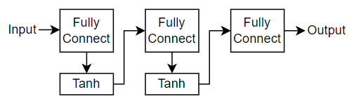
The function odeModel takes as input the function inputs t (unused) and y, and the ODE function parameters containing the convolution weights and biases. The function returns the output of a neural network with three fully connected layers with tanh operations between them.
The encoder and decoder use a neural ODE. A neural ODE is an ODE problem of the form where is a neural network with input and learnable parameters . In this case, the encoder and decoder neural ODE use the same neural network that consists of three fully connect operations with tanh activations between them.
This diagram shows the structure of the neural network.
function z = odeModel(~,y,parameters)

weights = parameters.fc1.Weights;
bias = parameters.fc1.Bias;
z = fullyconnect(y,weights,bias);
z = tanh(z);

weights = parameters.fc2.Weights;
bias = parameters.fc2.Bias;
z = fullyconnect(z,weights,bias);
z = tanh(z);

weights = parameters.fc3.Weights;
bias = parameters.fc3.Bias;
z = fullyconnect(z,weights,bias);

end
Mini-Batch Preprocessing Function
The preprocessMiniBatch function preprocesses the data using these steps:
Preprocess the predictors by using the
preprocessMiniBatchPredictorsfunction.Create a mini-batch of targets that matches the input data.
Randomly set 50 time steps of the sequence data to zero and create a mask indicating the missing values.
function [X,mask,T] = preprocessMiniBatch(XCell)

X = preprocessMiniBatchPredictors(XCell);
mask = true(size(X));
T = X;

% Remove time steps at random.
[~,numObservations,numTimestamps] = size(X);

for n = 1:numObservations
    idx = randsample(numTimestamps,50);
    idx = sort(idx);

    X(:,n,idx) = 0;
    mask(:,n,idx) = false;
end

end
Mini Batch Predictors Preprocessing Function
The preprocessMiniBatchPredictors function preprocesses the mini-batch predictors by extracting the sequence data from the input cell array and coverts it into a numeric array by concatenating the contents along the second dimension.
function X = preprocessMiniBatchPredictors(XCell)

X = cat(2,XCell{:});

end
Forward Euler Solver
The euler function takes as input the ODE function f, time internal t, input values y, ODE parameters, and the optional name-value argument MaxStepSize that specifies the step size to iterate over the interval. The function returns the forward Euler output. The forward Euler function is a fast ODE solver but is typically less accurate and less flexible than adaptive ODE solvers such as dlode45.
function y = euler(f,t,y,parameters,args)

arguments
    f
    t
    y
    parameters
    args.StepSize = 0.1;
end

stepSize = args.StepSize;

t1 = t(1);
t2 = t(2);
t2 = min(t2,t1 - stepSize);
tspan = t1:stepSize:t2;

y = y;

for i = 1:numel(tspan)-1
    y = y + (t(i+1)-t(i))*f(t,y,parameters);
end

end
Bibliography
[1] Chen, Ricky T. Q., Yulia Rubanova, Jesse Bettencourt, and David Duvenaud. “Neural Ordinary Differential Equations.” Preprint, submitted December 13, 2019. https://arxiv.org/abs/1806.07366
[2] Yulia Rubanova, Ricky T. Q. Chen, David Duvenaud. "Latent ODEs for Irregularly-Sampled Time Series" Preprint, submitted July 8, 2019. https://arxiv.org/abs/1907.03907
[3] Diederik P Kingma, Max Welling. "Auto-Encoding Variational Bayes." Preprint, submitted, submitted December 20, 2013. https://arxiv.org/abs/1312.6114
See Also
dlode45 | dlarray | dlfeval | dlgradient | fullyconnect | minibatchqueue | l2loss | gru
Topics
- Custom Loss Functions
- Custom Training Loops
- Custom Training Loop Model Loss Functions
- Train Neural ODE Network
- Dynamical System Modeling Using Neural ODE
- Train Neural ODE Network with Control Input
- Solve PDE Using Fourier Neural Operator
- Initialize Learnable Parameters for Model Function
- Specify Training Options in Custom Training Loop
- List of Functions with dlarray Support