Train Neural Network with Tabular Data
This example shows how to train a neural network with tabular data.
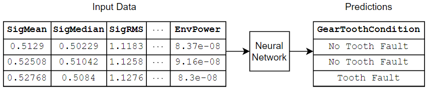
If you have a data set of numeric and categorical features (for example, tabular data without spatial or time dimensions), then you can train a deep neural network using a feature input layer. This example trains a neural network that predicts the gear tooth condition given a table of numeric and categorical sensor readings.
Load Training Data
Read the transmission casing data from the CSV file "transmissionCasingData.csv".
filename = "transmissionCasingData.csv";
tbl = readtable(filename,TextType="String");
Convert the labels for prediction to categorical using the convertvars function.
labelName = "GearToothCondition";
tbl = convertvars(tbl,labelName,"categorical");
View the class names of the data set.
classNames = categories(tbl.(labelName))
classNames = 2×1 cell
    {'No Tooth Fault'}
    {'Tooth Fault'   }
To train a network using categorical features, you must first convert the categorical features to the categorical data type. Convert the categorical predictors to categorical using the convertvars function by specifying a string array containing the names of all the categorical input variables. In this data set, there are two categorical features with names "SensorCondition" and "ShaftCondition".
categoricalPredictorNames = ["SensorCondition" "ShaftCondition"];
tbl = convertvars(tbl,categoricalPredictorNames,"categorical");
Set aside data for testing. Partition the data into a training set containing 80% of the data, a validation set containing 10% of the data, and a test set containing the remaining 10% of the data. To partition the data, use the trainingPartitions function, attached to this example as a supporting file. To access this file, open the example as a live script.
numObservations = size(tbl,1);
[idxTrain,idxValidation,idxTest] = trainingPartitions(numObservations,[0.80 0.1 0.1]);

tblTrain = tbl(idxTrain,:);
tblValidation = tbl(idxValidation,:);
tblTest = tbl(idxTest,:);
Define Neural Network Architecture
This example trains the neural network for categorical input features by one-hot encoding them. To specify the input size of the neural network, calculate the number of input features that includes the one-hot encoded categorical data. The number of features is the number of numeric columns of the training data plus the total number of categories among the categorical predictors.
numCategoricalPredictors = numel(categoricalPredictorNames);
numFeatures = size(tblTrain,2) - numCategoricalPredictors - 1;

for name = categoricalPredictorNames
    numCategories = numel(categories(tblTrain.(name)));
    numFeatures = numFeatures + numCategories;
end
Define the neural network architecture.
For feature input, specify a feature input layer with an input size that matches the number of features.
Specify a fully connected layer with a size of 16, followed by a layer normalization and ReLU layer.
For classification output, specify a fully connected layer with a size that matches the number of classes, followed by a softmax layer.
hiddenSize = 16;

numClasses = numel(classNames);

layers = [
    featureInputLayer(numFeatures)
    fullyConnectedLayer(hiddenSize)
    layerNormalizationLayer
    reluLayer
    fullyConnectedLayer(numClasses)
    softmaxLayer];
Specify Training Options
Specify the training options:
Train using the L-BFGS solver. This solver suits tasks with small networks and when the data fits in memory.
Train using the CPU. Because the network and data are small, the CPU is better suited.
One-hot encode the categorical inputs.
Validate the network every 5 iterations using the validation data.
Return the network with the lowest validation loss.
Display the training progress in a plot and monitor the accuracy metric.
Suppress the verbose output.
options = trainingOptions("lbfgs", ...
    ExecutionEnvironment="cpu", ...
    CategoricalInputEncoding="one-hot", ...
    ValidationData=tblValidation, ...
    ValidationFrequency=5, ...
    OutputNetwork="best-validation", ...
    Plots="training-progress", ...
    Metrics="accuracy", ...
    Verbose=false);
Train Neural Network
Train the neural network using the trainnet function. For classification, use cross-entropy loss.
[net,info] = trainnet(tblTrain,layers,"crossentropy",options);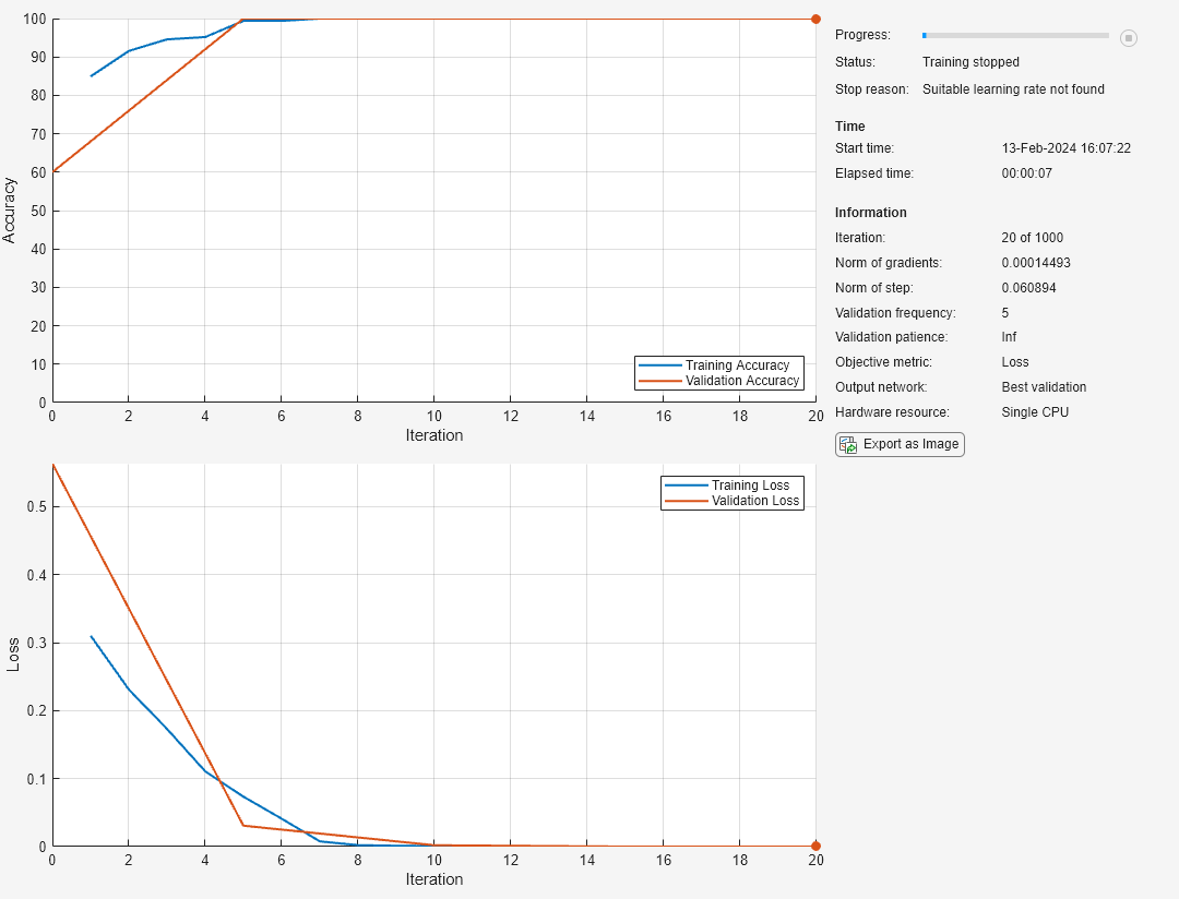
The plot shows the training and validation accuracy and loss. When training completes, the plot shows the stopping reason. When you use the L-BFGS solver, the stopping reason can show that the line search failed and that the software was unable to find a suitable learning rate. This scenario can happen when the solver reaches a minimal loss value quickly, or when the step and gradient norms are close to zero.
Test Neural Network
Predict the labels of the test data using the trained network. Predict the classification scores using the trained network then convert the predictions to labels using the onehotdecode function.
Test the neural network using the testnet function.
For single-label classification, evaluate the accuracy. The accuracy is the percentage of correct predictions.
One-hot encode the categorical inputs.
Test the neural network using the CPU.
accuracy = testnet(net,tblTest,"accuracy", ...
    CategoricalInputEncoding="one-hot", ...
    ExecutionEnvironment="cpu")
accuracy =
86.3636
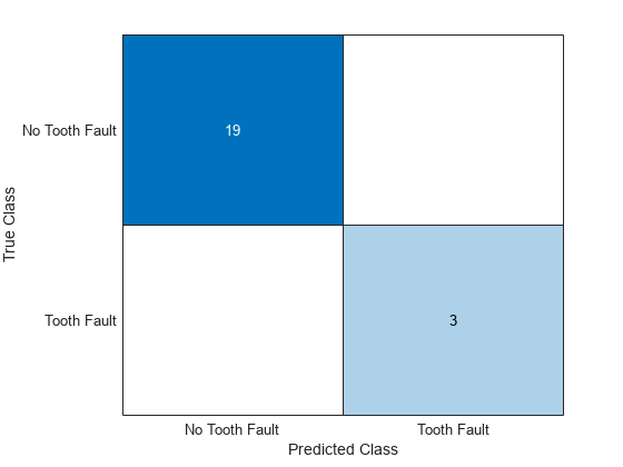
Visualize the predictions in a confusion chart by separating the targets from the test data, making predictions, and then converting the scores to labels.
Separate the targets from the data.
TTest = tblTest.(labelName);
Make predictions using the minibatchpredict function, and convert the classification scores to labels using the scores2label function.
One-hot encode the categorical inputs.
Make predictions using the CPU.
scoresTest = minibatchpredict(net,tblTest, ...
    CategoricalInputEncoding="one-hot", ...
    ExecutionEnvironment="cpu");

YTest = scores2label(scoresTest,classNames);
Visualize the predictions in a confusion chart.
confusionchart(TTest,YTest)
See Also
trainnet | trainingOptions | fullyConnectedLayer | Deep Network
Designer | featureInputLayer