Use parfeval to Train Multiple Deep Learning Networks
This example shows how to use parfeval to perform a parameter sweep on the depth of the network architecture for a deep learning network and retrieve data during training.
Deep learning training often takes hours or days, and searching for good architectures can be difficult. With parallel computing, you can speed up and automate your search for good models. If you have access to a machine with multiple graphical processing units (GPUs), you can complete this example on a local copy of the data set with a local parallel pool. If you want to use more resources, you can scale up deep learning training to the cloud.
You can use Experiment Manager to design and run experiments to train and compare deep learning networks, and run multiple trials at the same time in parallel. If you instead want to programmatically train multiple networks in parallel to perform a parameter sweep in the background without blocking MATLAB® and optionally stop early if results are satisfactory, you can use parfeval (Parallel Computing Toolbox).
This example shows how to use parfeval to perform a parameter sweep on the depth of a network architecture in a cluster in the cloud. You can modify the script to do a parameter sweep on any other parameter. Also, this example shows how to obtain feedback from the workers during computation by using a DataQueue object.
Requirements
Before you can run this example, you need to configure a cluster and upload your data to the Cloud. In MATLAB, you can create clusters in the cloud directly from the MATLAB Desktop. On the Home tab, in the Parallel menu, select Create and Manage Clusters. In the Cluster Profile Manager, click Create Cloud Cluster. Alternatively, you can use MathWorks Cloud Center to create and access compute clusters. For more information, see Getting Started with Cloud Center. For this example, ensure that your cluster is set as default on the MATLAB Home tab, in Parallel > Select a Default Cluster. After that, upload your data to an Amazon S3 bucket and use it directly from MATLAB. This example uses a copy of the CIFAR-10 data set that is already stored in Amazon S3. For instructions, see Work with Deep Learning Data in AWS.
Load Data Set from the Cloud
Load the training and test data sets from the cloud using imageDatastore. Split the training data set into training and validation sets, and keep the test data set to test the best network from the parameter sweep. In this example, you use a copy of the CIFAR-10 data set stored in Amazon S3. To ensure that the workers have access to the datastore in the cloud, make sure that the environment variables for the AWS credentials are set correctly. See Work with Deep Learning Data in AWS.
imds = imageDatastore("s3://cifar10cloud/cifar10/train", ...
    IncludeSubfolders=true, ...
    LabelSource="foldernames");

imdsTest = imageDatastore("s3://cifar10cloud/cifar10/test", ...
    IncludeSubfolders=true, ...
    LabelSource="foldernames");

[imdsTrain,imdsValidation] = splitEachLabel(imds,0.9);
Train the network with augmented image data by creating an augmentedImageDatastore object. Use random translations and horizontal reflections. Data augmentation helps prevent the network from overfitting and memorizing the exact details of the training images.
imageSize = [32 32 3];
pixelRange = [-4 4];
imageAugmenter = imageDataAugmenter( ...
    RandXReflection=true, ...
    RandXTranslation=pixelRange, ...
    RandYTranslation=pixelRange);
augmentedImdsTrain=augmentedImageDatastore(imageSize,imdsTrain, ...
    DataAugmentation=imageAugmenter, ...
    OutputSizeMode="randcrop");
Train Several Networks Simultaneously
Specify the training options. Set the mini-batch size and scale the initial learning rate linearly according to the mini-batch size. Set the validation frequency so that trainnet validates the network once per epoch.
miniBatchSize = 128;
initialLearnRate = 1e-1 * miniBatchSize/256;
validationFrequency = floor(numel(imdsTrain.Labels)/miniBatchSize);
options = trainingOptions("sgdm", ...
    MiniBatchSize=miniBatchSize, ... % Set the mini-batch size
    Verbose=false, ... % Do not send command line output.
    Metrics="accuracy", ...
    InitialLearnRate=initialLearnRate, ... % Set the scaled learning rate.
    L2Regularization=1e-10, ...
    MaxEpochs=30, ...
    Shuffle="every-epoch", ...
    ValidationData=imdsValidation, ...
    ValidationFrequency=validationFrequency);
Specify the depths for the network architecture on which to do a parameter sweep. Perform a parallel parameter sweep training several networks simultaneously using parfeval. Use a loop to iterate through the different network architectures in the sweep. Create the helper function createNetworkArchitecture at the end of the script, which takes an input argument to control the depth of the network and creates an architecture for CIFAR-10. Use parfeval to offload the computations performed by trainnet to a worker in the cluster. parfeval returns a future object to hold the trained networks and training information when computations are done.
By default, the trainnet function uses a GPU if one is available. Training on a GPU requires a Parallel Computing Toolbox™ license and a supported GPU device. For information on supported devices, see GPU Computing Requirements (Parallel Computing Toolbox). Otherwise, the trainnet function uses the CPU. To specify the execution environment, use the ExecutionEnvironment training option.
netDepths = 1:20;
numTrials = numel(netDepths);

for idx = 1:numTrials
    networksFuture(idx) = parfeval(@trainnet,2, ...
        augmentedImdsTrain,createNetworkArchitecture(netDepths(idx)),"crossentropy",options);
end
Starting parallel pool (parpool) using the 'myCloudCluster' profile ...
21-Jul-2025 13:25:23: Job Queued. Waiting for parallel pool job with ID 1 to start ...
Connected to parallel pool with 6 workers.
parfeval does not block MATLAB, which means you can continue executing commands. In this case, obtain the trained networks and their training information by using the fetchOutputs (Parallel Computing Toolbox) function on a future object. The fetchOutputs function retrieves the results from the specified future object in the networksFuture array. As using parfeval and fetchOutputs allows you to fetch intermediate results, you can define a stopping criteria. Query the validation accuracy after each network finishes training and cancel all network training if the accuracy has not increased for five consecutive trials. Return the network with the highest validation accuracy.
bestAccuracy = 0;
bestTrial = 0;

for idx = 1:numTrials
    [trainedNetwork,trainingInfo] = fetchOutputs(networksFuture(idx));

    validationHistory = trainingInfo.ValidationHistory;
    disp("Network " + idx + " validation accuracy: "+ validationHistory.Accuracy(end) + "%")

    if validationHistory.Accuracy(end) > bestAccuracy
        bestAccuracy = validationHistory.Accuracy(end);
        bestTrial = idx;
        bestNetwork = trainedNetwork;
    elseif idx - bestTrial == 5
        disp("Stopping training because validation accuracy hasn't improved for five consecutive trials.")
        disp("Best network: Network " + bestTrial + " (" + bestAccuracy + "%)")
        cancel(networksFuture)
        break
    end
end
Network 1 validation accuracy: 72.06%
Network 2 validation accuracy: 77.22%
Network 3 validation accuracy: 75.78%
Network 4 validation accuracy: 74.48%
Network 5 validation accuracy: 73.7%
Network 6 validation accuracy: 76.18%
Network 7 validation accuracy: 74.14%
Stopping training because validation accuracy hasn't improved for five consecutive trials.
Best network: Network 2 (77.22%)
Test the performance of the best network against the test data set. To make predictions with multiple observations, use the minibatchpredict function. To convert the prediction scores to labels, use the scores2label function. The minibatchpredict function automatically uses a GPU if one is available.
classNames = categories(imdsTest.Labels);
scores = minibatchpredict(bestNetwork,imdsTest);
Y = scores2label(scores,classNames);
accuracy = sum(Y == imdsTest.Labels)/numel(imdsTest.Labels)
accuracy =
0.7622
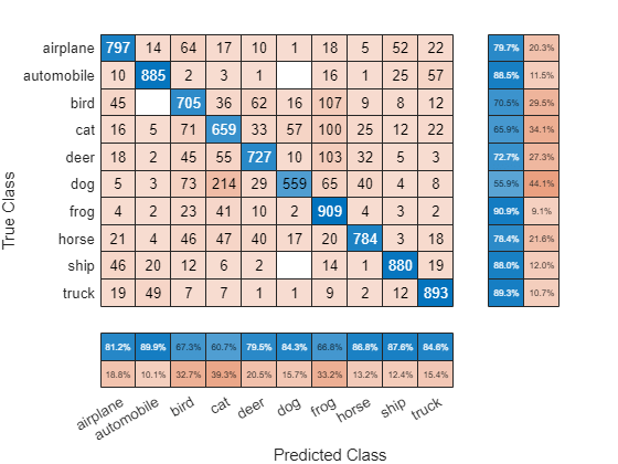
Calculate the confusion matrix for the test data.
figure
confusionchart(imdsTest.Labels,Y,RowSummary="row-normalized",ColumnSummary="column-normalized");
Send Feedback Data During Training
Prepare and initialize plots that show the training progress in each of the workers. Use animatedLine for a convenient way to show changing data. To avoid creating a large number of plots, hide each figure by setting the Visible property to "off". During training, you can choose which networks to monitor and set their Visible property to "on".
for idx = 1:numTrials
    fig(idx) = figure(Visible="off");
    xlabel("Iteration")
    ylabel("Training Accuracy")
    title("Network " + idx)
    grid on
    ylim([0 100])
    lines(idx) = animatedline;
end
Send the training progress data from the workers to the client by using DataQueue, and then plot the data. Update the plots each time the workers send training progress feedback by using afterEach. The parameter opts contains information about the worker, training iteration, and training accuracy.
D = parallel.pool.DataQueue;
afterEach(D, @(opts) updatePlot(lines,opts{:}));
Specify the depths for the network architecture on which to do a parameter sweep, and perform the parallel parameter sweep using parfeval. Allow the workers to access any helper function in this script, by adding the script to the current pool as an attached file. Define an output function in the training options to send the training progress from the workers to the client. The training options depend on the index of the worker and must be included inside the for loop.
addAttachedFiles(gcp,mfilename);

miniBatchSize = 128;
initialLearnRate = 1e-1 * miniBatchSize/256; % Scale the learning rate according to the mini-batch size.
validationFrequency = floor(numel(imdsTrain.Labels)/miniBatchSize);

options = trainingOptions("sgdm", ...
    MiniBatchSize=miniBatchSize, ... % Set the corresponding MiniBatchSize in the sweep.
    Verbose=false, ... % Do not send command line output.
    InitialLearnRate=initialLearnRate, ... % Set the scaled learning rate.
    Metrics="accuracy", ...
    L2Regularization=1e-10, ...
    MaxEpochs=30, ...
    Shuffle="every-epoch", ...
    ValidationData=imdsValidation, ...
    ValidationFrequency=validationFrequency);

for idx = 1:numel(netDepths)
    options.OutputFcn=@(state) sendTrainingProgress(D,idx,state); % Set an output function to send intermediate results to the client.

    networksFuture(idx) = parfeval(@trainnet,2, ...
        augmentedImdsTrain,createNetworkArchitecture(netDepths(idx)),"crossentropy",options);
end
parfeval invokes trainnet on a worker in the cluster. Computations happen on the background, so you can continue working in MATLAB. If you want to stop a parfeval computation, you can call cancel on its corresponding future variable. For example, if you observe that a network is underperforming, you can cancel its future. When you do so, the next queued future variable starts its computations.
Display the training progress plot for the first network.
fig(1).Visible = "on";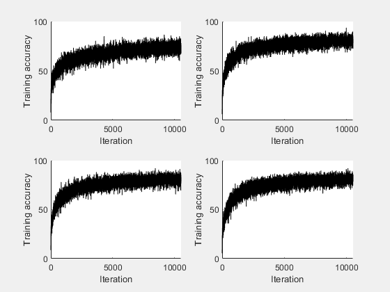
Return the network with the highest validation accuracy and cancel all network training if the accuracy has not increased for five consecutive trials.
bestAccuracy = 0;
bestTrial = 0;

for idx = 1:numTrials
    [trainedNetwork,trainingInfo] = fetchOutputs(networksFuture(idx));

    validationHistory = trainingInfo.ValidationHistory;
    disp("Network " + idx + " validation accuracy: "+ validationHistory.Accuracy(end) + "%")

    if validationHistory.Accuracy(end) > bestAccuracy
        bestAccuracy = validationHistory.Accuracy(end);
        bestTrial = idx;
        bestNetwork = trainedNetwork;
    elseif idx - bestTrial == 5
        disp("Stopping training because validation accuracy hasn't improved for five consecutive trials.")
        disp("Best network: Network " + bestTrial + " (" + bestAccuracy + "%)")
        cancel(networksFuture)
        break
    end
end
Network 1 validation accuracy: 73.56%
Network 2 validation accuracy: 75.78%
Network 3 validation accuracy: 76.1%
Network 4 validation accuracy: 74.9%
Network 5 validation accuracy: 74.76%
Network 6 validation accuracy: 77.14%
Network 7 validation accuracy: 74.2%
Network 8 validation accuracy: 73.66%
Network 9 validation accuracy: 66.4%
Network 10 validation accuracy: 66.64%
Network 11 validation accuracy: 69.4%
Stopping training because validation accuracy hasn't improved for five consecutive trials.
Best network: Network 6 (77.14%)
Helper Functions
Define a network architecture for the CIFAR-10 data set with a function, and use an input argument to adjust the depth of the network. To simplify the code, use convolutional blocks that convolve the input. The pooling layers downsample the spatial dimensions.
function layers = createNetworkArchitecture(netDepth)
imageSize = [32 32 3];
netWidth = round(16/sqrt(netDepth)); % netWidth controls the number of filters in a convolutional block

layers = [
    imageInputLayer(imageSize)

    convolutionalBlock(netWidth,netDepth)
    maxPooling2dLayer(2,Stride=2)
    convolutionalBlock(2*netWidth,netDepth)
    maxPooling2dLayer(2,Stride=2)
    convolutionalBlock(4*netWidth,netDepth)
    averagePooling2dLayer(8)

    fullyConnectedLayer(10)
    softmaxLayer
    ];
end
Define a function to create a convolutional block in the network architecture.
function layers = convolutionalBlock(numFilters,numConvLayers)
layers = [
    convolution2dLayer(3,numFilters,Padding="same")
    batchNormalizationLayer
    reluLayer
    ];

layers = repmat(layers,numConvLayers,1);
end
Define a function to send the training progress to the client through DataQueue.
function stop = sendTrainingProgress(D,idx,info)
if info.State == "iteration" && ~isempty(info.TrainingAccuracy)
    send(D,{idx,info.Iteration,info.TrainingAccuracy});
end
stop = false;
end
Define an update function to update the plots when a worker sends an intermediate result.
function updatePlot(lines,idx,iter,acc)
addpoints(lines(idx),iter,acc);
drawnow limitrate
end
See Also
parfeval (Parallel Computing Toolbox) | afterEach | trainnet | trainingOptions | dlnetwork | imageDatastore