Deep Signal Anomaly Detector
Libraries:
DSP System Toolbox /
AI
Description
The Deep Signal Anomaly Detector block detects real-time signal anomalies in Simulink® using a trained long short-term memory (LSTM) autoencoder or a trained long short-term memory (LSTM) forecaster (since R2024b) deep learning network model.
You must first create and train a detector object in MATLAB® using the deepSignalAnomalyDetector function, and then configure the block to use this
model in Simulink. To configure the block, specify the path to the detector model in the block
dialog box. For more information on these steps, see User Workflow.
Note
This block additionally requires a Deep Learning Toolbox™ license.
Examples
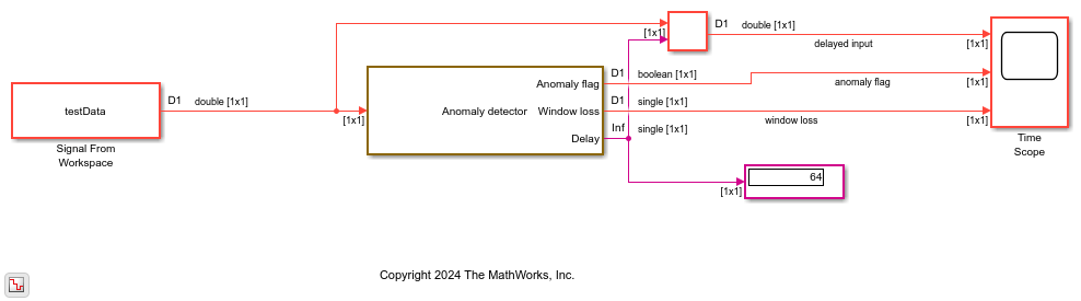
Use the Deep Signal Anomaly Detector block to detect anomalies in a sinusoidal signal. The block uses a detector that has been trained on a set of sinusoidal signals of constant frequency and amplitude. Use the time scope to plot the input, anomaly flag, and the window loss.
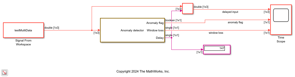
Open the detectAnomaliesSingleChannel.slx model. The input is a single-channel sinusoidal signal. The Deep Signal Anomaly Detector block reads the post-processing parameters from the detector MAT-file. As you can see in the Parameter values from MAT-file section in the block dialog box, the window length WL is 1 and the overlap length OL is 0. The hop size  is 1. The threshold value is approximately 0.06.
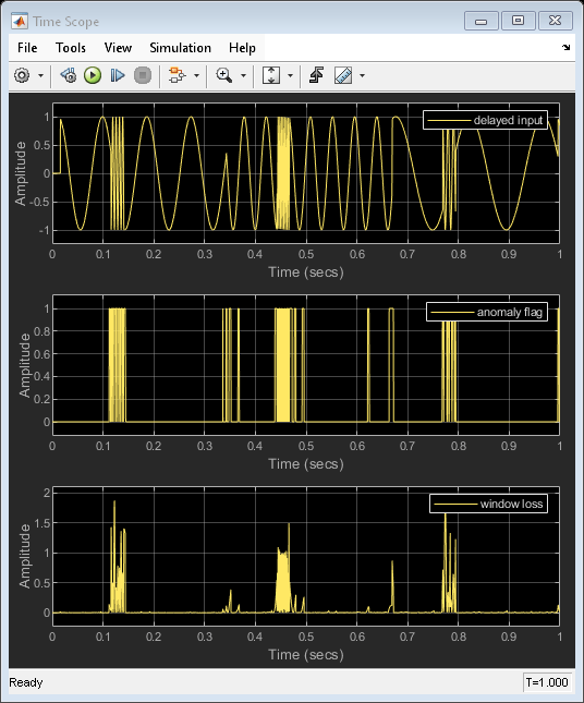
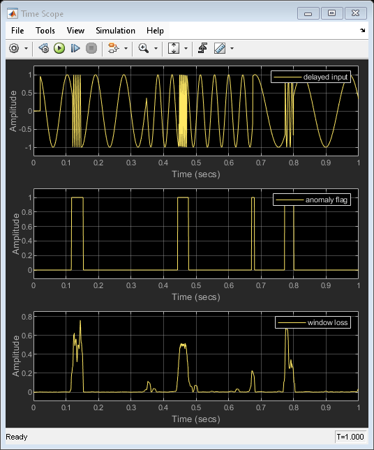
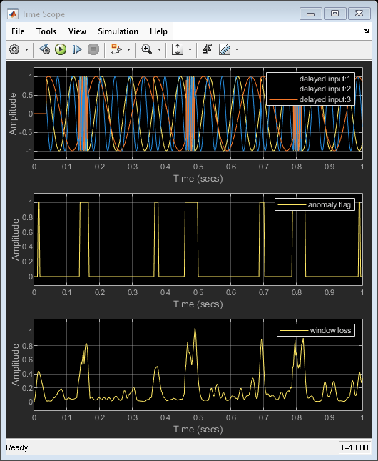
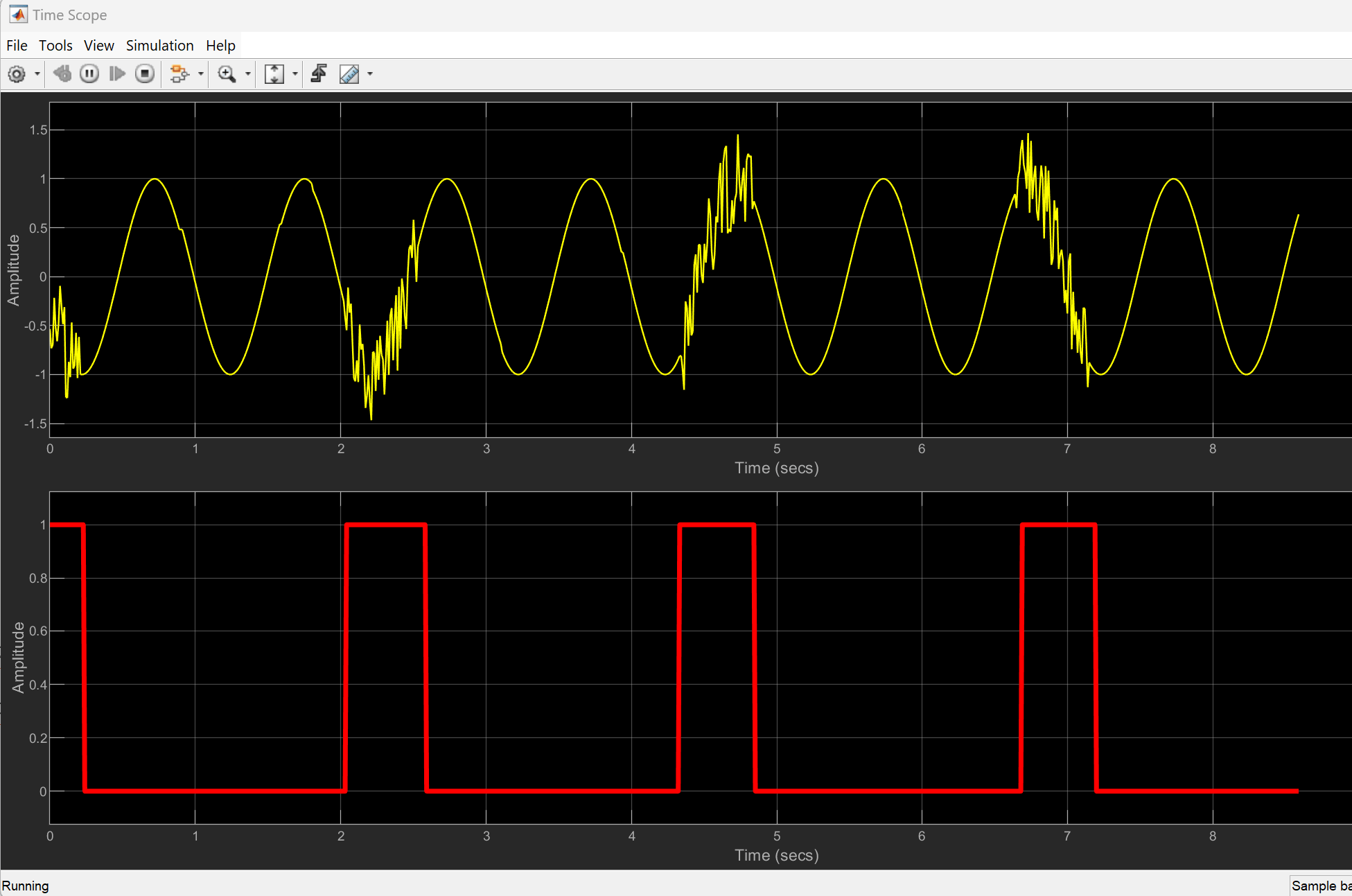
Run the model. The first plot shows the delayed input signal. The delay value is equal to the number of samples the Deep Signal Anomaly Detector block outputs through the Delay port. To align the input with the anomaly flag and window loss, use a Delay block, set the Delay length parameter to Input, and provide the delay estimate as the delay input to the Delay block.
The second plot shows the anomalies in the signal. A value of 1 indicates the presence of an anomaly. The third plot shows the aggregate window loss.
When the window loss is greater than the threshold, the block flags the region as having an anomaly. In this case, since the window length is 1, the block detects point anomalies. The block turns on the anomaly flag for every sample where the window loss is greater than the threshold value. This makes the anomaly plot look very noisy.
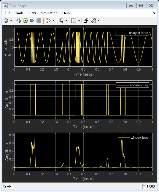
Increasing Window Length
To make the anomaly plot look less noisy, increase the window length in the Deep Signal Anomaly Detector block to 40. To do that, set the Parameters for post-processing parameter to Specify on dialog. Set Window length to 40 and Overlap length to 39. Set the threshold to the default value obtained from the MAT-file.
Run the model. The anomaly plot looks much smoother. However, there are still some regions where the window loss value is low (around 0.1) and the block detects these regions as anomalies.
Increasing Threshold
To filter out anomalies that have a relatively lower window loss, increase the threshold value to 0.15. To be called an anomaly, the aggregate window loss must now be greater than 0.15. Increasing the threshold value removes the unintended anomaly detections and further smoothens the plot.
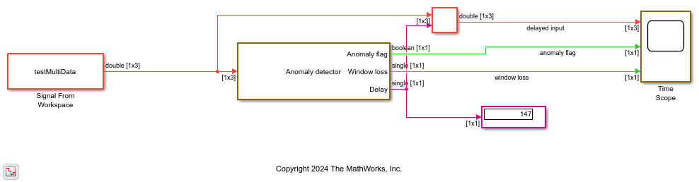
Open the detectAnomaliesMultiChannel.slx model.
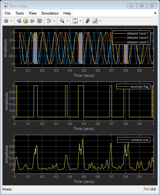
The input is a multichannel sinusoidal signal. If one of the channels has an anomaly, the Deep Signal Anomaly Detector block assumes the presence of the anomaly across all input channels and returns a scalar value at the Anomaly flag port. The block uses a window length WL of 40 and an overlap length OL of 39. The hop size  is 1.
is 1.
Run the model. The first plot shows the delayed input signal. The second plot shows the presence of an anomaly in the signal. The third plot shows the corresponding aggregate window loss.
Observe from the time scope that the presence of an anomaly is uniform across all channels and the block provides a single-channel output for the window loss and anomaly flag, corresponding to all the channels of the input.
The sample time of the input and output ports is the same. You can confirm this from the color of the signals in the model. The delay port always has a constant sample time.
Changing Hop Size
Change the hop size in the Deep Signal Anomaly Detector block and note the effect on the sample time of the output ports Anomaly flag and Window loss.
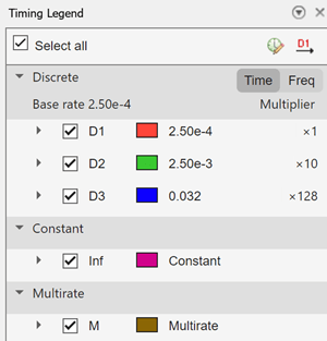
Decrease the overlap length to 30. The hop size is now 10. Run the model again. View the sample time of the two output ports in the timing legend. To view the timing legend, in the Debug tab of the Simulink model toolstrip, click Information Overlays > Timing Legend. The timing legend shows that the sample time of the output ports is 10 times the sample time of the input port. For every 10 input samples, the block produces 1 output sample. To change the sample time at the output port, adjust the hop size accordingly. For more information on sample time at the block ports, see Sample- and Frame-Based Concepts.
Since R2024b
This example trains the LSTM forecaster network model and imports the model into a Deep Signal Anomaly Detector block. The Deep Signal Anomaly Detector block assumes that for multichannel inputs, the presence of anomaly is uniform across channels. To detect anomalies in multichannel signals where the presence of anomaly in each channel is uncorrelated, you can use a separate block for each channel of input. This example uses two such blocks to detect anomalies in the two channels of the input sinusoidal signal.
Train Model
Load the train and test data file sineWaveData.mat. The train data contains 40 single-channel sinusoidal signals of different frequencies with no noise. The test data contains two-channel sinusoidal signal with noise or anomaly. The presence of an anomaly is independent on both channels.
Train the deep signal anomaly detector model using the 'lstmforecaster' method. Export the saved detector model and parameters to the LSTMForecasterModel MAT file. This MAT file is provided with the example.
You can use this code to train the detector model using the train data.
load sineWaveData.mat
plot(dataTest);
anomalyDetector =  deepSignalAnomalyDetector(1,'lstmforecaster',WindowLength=10);
opts = trainingOptions("adam",MaxEpochs=300);
trainDetector(anomalyDetector,dataTrain,opts)
saveModel(anomalyDetector,'LSTMForecasterModel');
Open and Run Model
Open the detectIndependentAnomalies Simulink model. The two Deep Signal Anomaly Detector blocks in the model import the LSTMForecasterModel MAT file. The blocks also import post-processing parameters such as the window length, overlap length, threshold, and window loss aggregation from the MAT file. The input to the model is the test data which contains independent anomalies on both its channels.
Run the detectIndependentAnomalies Simulink model. The two Deep Signal Anomaly Detector blocks detect anomalies in the two input channels separately and return a scalar value at the Anomaly flag port. The first plot shows the two channels of the sinusoidal signal with the anomalies. The second plot shows the output of the Anomaly flag port. As you can see, the LSTM forecaster model accurately detects the presence of an anomaly on both the channels.


Extended Examples
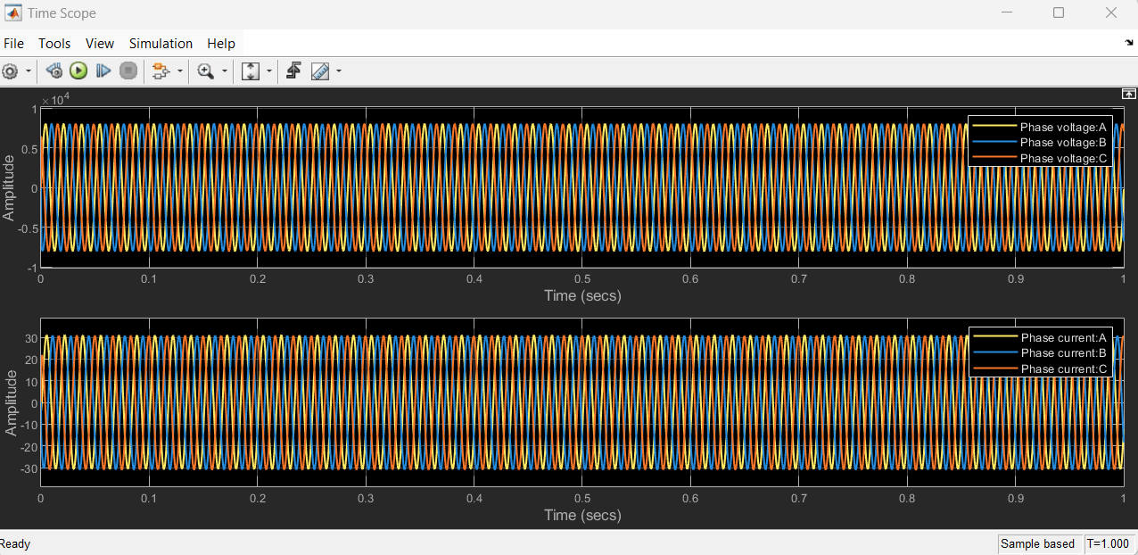
Fault Detection and Localization in Three-Phase Power Transmission Using Deep Signal Anomaly Detector in Simulink
Detect faults in three-phase power transmission using the Deep Signal Anomaly Detector block.
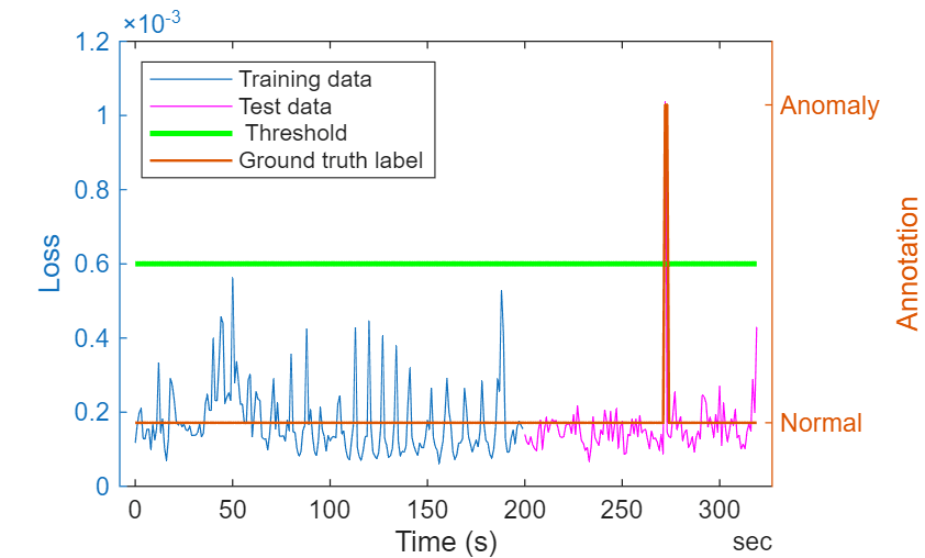
Detect Anomalies in ECG Data Using Wavelet Scattering and LSTM Autoencoder in Simulink
Use wavelet scattering and deep learning network to detect anomalies in ECG signals.
Real-Time Noise Detection on Raspberry Pi Using Deep Signal Anomaly Detector
Detect the presence of noise on a Raspberry Pi device.
Ports
Input
Output
Parameters
Block Characteristics
Data Types |
|
Direct Feedthrough |
|
Multidimensional Signals |
|
Variable-Size Signals |
|
Zero-Crossing Detection |
|
More About
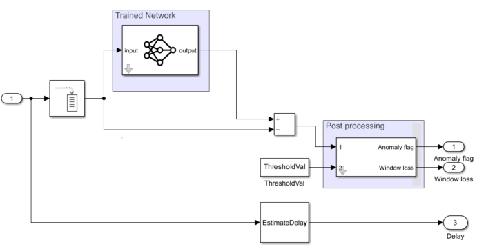
Algorithms
The Deep Signal Anomaly Detector block first buffers the input into frames and then tries to reconstruct the buffered signal using the trained network. The block processes the difference between the input and the reconstructed frames to obtain the window loss and anomaly flags. The block can also output an estimate of the delay (in samples) the input signal goes through as the trained network reconstructs this signal. For the LSTM Forecaster model, the block omits the buffering of the input signal, thereby reducing the delay added to the input signal. (since R2024b)