designMultistageInterpolator

Initialization

Choose an interpolation factor of 48, input sample rate of 640 kHz, one-sided bandwidth of 100 kHz, and a stopband attenuation of 90 dB.

L = 48;
Fin = 640e3;
Astop = 90;
BW = 1e5;

Compute the transition width using the following relationship:

Fc = Fin/2;
TW = 2*(Fc-BW);

Using the designMultirateFIR Function

Designing the interpolation filter using the designMultirateFIR function yields a single-stage design.

d = designMultirateFIR(InterpolationFactor=L,TransitionWidth=TW/(Fin*L/2),...
    StopbandAttenuation=Astop,SystemObject=true)

d = 
  dsp.FIRInterpolator with properties:

    InterpolationFactor: 48
        NumeratorSource: 'Property'
              Numerator: [3.6296e-05 3.9057e-05 4.0435e-05 4.0103e-05 3.7714e-05 3.2899e-05 2.5275e-05 1.4445e-05 0 -1.8471e-05 -4.1383e-05 -6.9142e-05 -1.0215e-04 -1.4078e-04 -1.8540e-04 -2.3633e-04 -2.9386e-04 -3.5824e-04 ... ] (1x401 double)

  Use get to show all properties

Compute the cost of implementing the interpolator. The interpolation filter requires 376 coefficients and 7 states. The number of multiplications per input sample and additions per input sample are 376 and 329, respectively.

cost(d)

ans = struct with fields:
                  NumCoefficients: 392
                        NumStates: 8
    MultiplicationsPerInputSample: 392
          AdditionsPerInputSample: 345

Using the designMultistageInterpolator Function

Design a multistage interpolator with the same filter specifications as the single-stage design.

By default, the number of stages given by the NumStages argument is set to 'auto', yielding an optimal design that tries to minimize the number of multiplications per input sample.

c = designMultistageInterpolator(L,Fin,TW,Astop)

c = 
  dsp.FilterCascade with properties:

         Stage1: [1x1 dsp.FIRInterpolator]
         Stage2: [1x1 dsp.FIRInterpolator]
    CloneStages: false

Calling the info function on c shows that the filter is implemented as a cascade of two dsp.FIRInterpolator objects with interpolation factors of 24 and 2, respectively.

Compute the cost of implementing the interpolator.

cost(c)

ans = struct with fields:
                  NumCoefficients: 184
                        NumStates: 12
    MultiplicationsPerInputSample: 322
          AdditionsPerInputSample: 275

The NumCoefficients and the MultiplicationsPerInputSample parameters are lower for the two-stage filter designed by the designMultistageInterpolator function, making it more efficient.

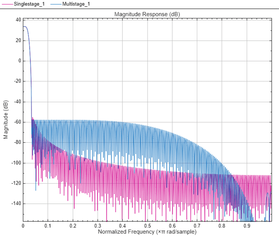
Compare the magnitude response of both designs.

filterAnalyzer(d,c,FilterNames=["Singlestage","Multistage"]);

The magnitude response shows that the transition width of both the filters is the same, making the filters comparable. The cost function shows that implementing the multistage design is more efficient compared to implementing the single-stage design.

Using the 'design' Option in the designMultistageInterpolator Function

The filter can be made even more efficient by setting the 'CostMethod' argument of the designMultistageInterpolator function to 'design'. By default, this argument is set to 'estimate'.

In the 'design' mode, the function designs each stage and computes the filter order. This yields an optimal design compared to the 'estimate' mode, where the function estimates the filter order for each stage and designs the filter based on the estimate.

Note that the 'design' option can take much longer compared to the 'estimate' option.

cOptimal = designMultistageInterpolator(L,Fin,TW,Astop,CostMethod='design')

cOptimal = 
  dsp.FilterCascade with properties:

         Stage1: [1x1 dsp.FIRInterpolator]
         Stage2: [1x1 dsp.FIRInterpolator]
         Stage3: [1x1 dsp.FIRInterpolator]
    CloneStages: false

cost(cOptimal)

ans = struct with fields:
                  NumCoefficients: 74
                        NumStates: 17
    MultiplicationsPerInputSample: 296
          AdditionsPerInputSample: 249

Initialization

Choose an interpolation factor of 24, input sample rate of 250 Hz, stopband attenuation of 90 dB, and a transition width of 0.03$\times$(Fs$\times$L)/2.

L = 24;
Fs = 250;
Astop = 90;
TW = 0.03*Fs*L/2;

Design the Filter

Design the two filters using the designMultistageInterpolator function.

cAuto = designMultistageInterpolator(L,Fs,TW,Astop,NumStages="auto")

cAuto = 
  dsp.FilterCascade with properties:

         Stage1: [1x1 dsp.FIRInterpolator]
         Stage2: [1x1 dsp.FIRInterpolator]
         Stage3: [1x1 dsp.FIRInterpolator]
    CloneStages: false

cTwo = designMultistageInterpolator(L,Fs,TW,Astop,NumStages=2)

cTwo = 
  dsp.FilterCascade with properties:

         Stage1: [1x1 dsp.FIRInterpolator]
         Stage2: [1x1 dsp.FIRInterpolator]
    CloneStages: false

View the filter information using the info function. The 'auto' configuration designs a cascade of three FIR interpolators with interpolation factors 4, 3, and 2, respectively. The two-stage configuration designs a cascade of two FIR interpolators with interpolation factors 6 and 4, respectively.

Compare the Cost

Compare the cost of implementing the two designs using the cost function.

cost(cAuto)

ans = struct with fields:
                  NumCoefficients: 70
                        NumStates: 28
    MultiplicationsPerInputSample: 190
          AdditionsPerInputSample: 167

cost(cTwo)

ans = struct with fields:
                  NumCoefficients: 98
                        NumStates: 22
    MultiplicationsPerInputSample: 208
          AdditionsPerInputSample: 185

The 'auto' configuration interpolation filter yields a three-stage design that out-performs the two-stage design in terms of NumCoefficients and MultiplicationsPerInputSample metrics.