dsp.AllpassFilter

Single section or cascaded allpass filter

Description

The dsp.AllpassFilter object filters each channel of the input using allpass filter implementations. To import this object into Simulink^®, use the MATLAB^® System block.

To filter each channel of the input:

Create the dsp.AllpassFilter object and set its properties.
Call the object with arguments, as if it were a function.

To learn more about how System objects work, see What Are System Objects?

Creation

Syntax

Allpass = dsp.AllpassFilter

Allpass = dsp.AllpassFilter(Name=Value)

Description

Allpass = dsp.AllpassFilter returns an allpass filter System object™, Allpass, that filters each channel of the input signal independently using an allpass filter, with the default structure and coefficients.

Allpass = dsp.AllpassFilter(Name=Value) returns an allpass filter System object, Allpass, with each property set to the specified value by one or more Name-Value pair arguments. Name is the property name and Value is the corresponding value. For example, Structure='Lattice' sets the filter structure to 'Lattice'.

example

Properties

expand all

Unless otherwise indicated, properties are nontunable, which means you cannot change their values after calling the object. Objects lock when you call them, and the release function unlocks them.

If a property is tunable, you can change its value at any time.

For more information on changing property values, see System Design in MATLAB Using System Objects.

`Structure` — Internal allpass filter structure
`'Minimum multiplier'` (default) | `'Lattice'` | `'Wave Digital Filter'`

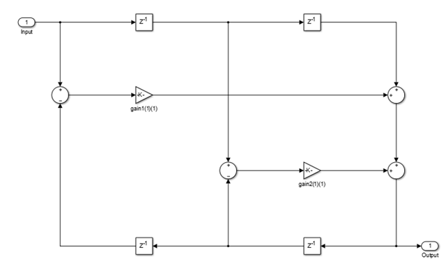
Internal allpass filter implementation structure, specified as one of these:

'Minimum multiplier'
'Lattice'
'Wave Digital Filter'

Each structure uses a different set of coefficients, independently stored in the corresponding object property.

`AllpassCoefficients` — Allpass polynomial coefficients
`[-2^(-1/2) 0.5]` (default) | N-by-1 | N-by-2 | N-by-4

Real allpass polynomial filter coefficients, specified as one of these:

N-by-1 matrix –– N first-order allpass sections.
N-by-2 matrix –– N second-order allpass sections.
N-by-4 matrix –– N fourth-order allpass sections. (since R2024a)

The default value of [-2^(-1/2) 0.5] defines a stable second-order allpass filter with poles and zeros located at ±π/3 in the z-plane.

Tunable: Yes

Dependencies

To enable this property, set the Structure property to 'Minimum multiplier'.

`WDFCoefficients` — Wave Digital Filter allpass coefficients
[`1/2, -2^(1/2)/3`] (default) | N-by-1 | N-by-2

Real allpass coefficients in the Wave Digital Filter form, specified as an N-by-1 or N-by-2 matrix of N first-order or second-order allpass sections. All elements must have absolute values less than or equal to 1. This value is a transformed version of the default value of AllpassCoefficients, computed using allpass2wdf(AllpassCoefficients). These coefficients define the same stable second-order allpass filter as when Structure is set to 'Minimum multiplier'.

Tunable: Yes

Dependencies

To enable this property, set the Structure property to 'Wave Digital Filter'.

`LatticeCoefficients` — Lattice allpass coefficients
`[-2^(1/2)/3, 1/2]` (default) | vector

Real or complex allpass coefficients as lattice reflection coefficients, specified as a row vector (single-section configuration) or a column vector. This value is a transformed and transposed version of the default value of AllpassCoefficients, computed using transpose(tf2latc([1 h.AllpassCoefficients])). These coefficients define the same stable second-order allpass filter as when Structure is set to 'Lattice'.

Tunable: Yes

Dependencies

To enable this property, set the Structure property to 'Lattice'.

`TrailingFirstOrderSection` — Indicate if last section is first order
`false` (default) | `true`

Indicate if last section is first order. When you set the TrailingFirstOrderSection property to true, the last section is considered to be first-order, and the second order term in the last row of the N-by-2 matrix is ignored. In case of the minimum multiplier structure, if you specify an N-by-4 matrix, this property has no effect on the filter coefficients.

Dependencies

To enable this property, set the Structure property to 'Minimum multiplier' or 'Wave Digital Filter'.

Usage

Syntax

y = Allpass(x)

Description

y = Allpass(x) filters the input signal x using an allpass filter to produce the output y. Each column of x is filtered independently as a separate channel over time.

example

Input Arguments

expand all

`x` — Data input
vector | matrix

Data input, specified as a vector or a matrix. This object also accepts variable-size inputs. Once the object is locked, you can change the size of each input channel, but you cannot change the number of channels.

Data Types: single | double
Complex Number Support: Yes

Output Arguments

expand all

`y` — Filtered output
vector | matrix

Filtered output, returned as a vector or a matrix. The size, data type, and complexity of the output signal matches that of the input signal.

Data Types: double | single
Complex Number Support: Yes

Object Functions

To use an object function, specify the System object as the first input argument. For example, to release system resources of a System object named obj, use this syntax:

release(obj)

expand all

Specific to `dsp.AllpassFilter`

`freqz`	Frequency response of discrete-time filter System object
`filterAnalyzer`	Analyze filters with Filter Analyzer app
`impz`	Impulse response of discrete-time filter System object
`info`	Information about filter System object
`coeffs`	Returns the filter System object coefficients in a structure
`cost`	Estimate cost of implementing filter System object
`grpdelay`	Group delay response of discrete-time filter System object
`outputDelay`	Determine output delay of single-rate or multirate filter

Common to All System Objects

`step`	Run System object algorithm
`release`	Release resources and allow changes to System object property values and input characteristics
`reset`	Reset internal states of System object

Examples

collapse all

Lowpass Filtering using Two Allpass Filters

Open Script

Construct the two dsp.AllpassFilter objects.

Fs  = 48000;    % in Hz
FL = 1024;
APF1 = dsp.AllpassFilter(AllpassCoefficients=[-0.710525516540603 0.208818210000029]);
APF2 =  dsp.AllpassFilter(AllpassCoefficients=[-0.940456403667957 0.6;...
    -0.324919696232907 0],...
    TrailingFirstOrderSection=true);

Construct the Transfer Function Estimator to estimate the transfer function between the random input and the Allpass filtered output.

TFE = dsp.TransferFunctionEstimator(FrequencyRange='onesided',...
    SpectralAverages=2);

Construct the dsp.ArrayPlot object to plot the magnitude response.

AP = dsp.ArrayPlot(PlotType='Line',YLimits=[-80 5],...
    YLabel='Magnitude (dB)',SampleIncrement=Fs/FL,...
    XLabel='Frequency (Hz)',Title='Magnitude Response',...
    ShowLegend=true,ChannelNames={'Magnitude Response'});

Filter the Input and show the magnitude response of the estimated transfer function between the input and the filtered output.

tic;
while toc < 5
    in  = randn(FL,1);
    out = 0.5.*(APF1(in) + APF2(in));
    A = TFE(in, out);
    AP(db(A));
end

Design and Implement Quasilinear IIR Halfband Filter

Since R2024a

Open Live Script

Design a quasi-linear IIR halfband filter with the order of 32 using the designHalfbandIIR function. Assign the filter coefficients to a coupled allpass filter.

[a0,a1] = designHalfbandIIR(FilterOrder=32,DesignMethod="quasilinphase",Verbose=true)

designHalfbandIIR(FilterOrder=32, TransitionWidth=0.1, DesignMethod="quasilinphase", Structure="single-rate", Datatype="double", SystemObject=false)

a0 = 4×4

     0     0     0     0
     0     0     0     0
     0     0     0     0
     0     0     0     0

a1 = 4×4

         0    0.8085         0    0.3051
         0    0.0387         0    0.2695
         0   -0.7054         0    0.2604
         0    0.3546         0   -0.4386

Construct the corresponding coupled allpass filter using the cascade and parallel functions. Alternatively, if you set the SystemObject argument of the designHalfbandIIR function to true, the function designs the same object.

B0 = dsp.AllpassFilter(AllpassCoefficients=a0);
B1 = dsp.AllpassFilter(AllpassCoefficients=a1);
filtObj = cascade(parallel(B0,cascade(dsp.Delay, B1)),0.5)

filtObj = 
  dsp.FilterCascade with properties:

         Stage1: [1x1 dsp.ParallelFilter]
         Stage2: 0.5000
    CloneStages: true

Create a dsp.DynamicFilterVisualizer object and visualize the magnitude response of the filter.

dfv = dsp.DynamicFilterVisualizer(NormalizedFrequency=true);
dfv(filtObj);

A quasi-linear IIR filter has a fairly constant group delay (hence almost linear phase) in the passband region of the filter.

grpdelay(filtObj)

Figure contains an axes object. The axes object with title Group Delay, xlabel Normalized Frequency ( times pi blank rad/sample), ylabel Group delay (samples) contains an object of type line.

phasez(filtObj)

Figure contains an axes object. The axes object with title Phase Response, xlabel Normalized Frequency ( times pi blank rad/sample), ylabel Phase (radians) contains an object of type line.

Create a spectrumAnalyzer object to visualize the spectra of the input and output signals.

scope = spectrumAnalyzer(SampleRate=2, ...
    PlotAsTwoSidedSpectrum=false,...
    ChannelNames=["Input Signal","Filtered Signal"]);

Stream in a noisy sinusoidal signal and filter the signal using the IIR halfband filter. The sinusoidal tone falls in the passband frequency of the filter and is therefore unaffected.

sine = dsp.SineWave(Frequency=1000,SampleRate=44100,SamplesPerFrame=1024)

sine = 
  dsp.SineWave with properties:

          Amplitude: 1
          Frequency: 1000
        PhaseOffset: 0
      ComplexOutput: false
             Method: 'Trigonometric function'
    SamplesPerFrame: 1024
         SampleRate: 44100
     OutputDataType: 'double'

for i = 1:1000
    x = sine()+0.005*randn(1024,1);
    y = filtObj(x);
    scope(x,y);
end

Design and Implement Butterworth IIR Halfband Filter

Open Live Script

Design a Butterworth IIR halfband filter with the order of 13 and construct the corresponding coupled allpass filter using the designHalfbandIIR function. Set the SystemObject argument of the function to true.

filtObj = designHalfbandIIR(FilterOrder=13,Verbose=true,SystemObject=true)

designHalfbandIIR(FilterOrder=13, DesignMethod="butter", Structure="single-rate", Datatype="double", SystemObject=true, Passband="lowpass")

filtObj = 
  dsp.FilterCascade with properties:

         Stage1: [1x1 dsp.ParallelFilter]
         Stage2: 0.5000
    CloneStages: true

Create a dsp.DynamicFilterVisualizer object and visualize the magnitude response of the filter.

dfv = dsp.DynamicFilterVisualizer(NormalizedFrequency=true);
dfv(filtObj);

Create a spectrumAnalyzer object to visualize the spectra of the input and output signals.

scope = spectrumAnalyzer(SampleRate=2, ...
    PlotAsTwoSidedSpectrum=false,...
    ChannelNames=["Input Signal","Filtered Signal"]);

Stream in random data and filter the signal using the IIR halfband filter.

for i = 1:1000
    x = randn(1024, 1);
    y = filtObj(x);
    scope(x,y);
end

Algorithms

expand all

The transfer function of an allpass filter is given by

$H (z) = \frac{c (n) + c (n - 1) z^{- 1} + ... + z^{- n}}{1 + c (1) z^{- 1} + ... + c (n) z^{- n}}$ .

c is allpass polynomial coefficients vector. The order, n, of the transfer function is the length of vector c.

In the minimum multiplier form and wave digital form, the allpass filter is implemented as a cascade of either second-order (biquad) sections or first-order sections. When the coefficients are specified as an N-by-2 matrix, each row of the matrix specifies the coefficients of a second-order filter. The last element of the last row can be ignored based on the trailing first-order setting. When the coefficients are specified as an N-by-1 matrix, each element in the matrix specifies the coefficient of a first-order filter. The cascade of all the filter sections forms the allpass filter.

In the lattice form, the coefficients are specified as a vector.

These structures are computationally more economical and structurally more stable compared to the generic IIR filters, such as df1, df1t, df2, df2t. For all structures, the allpass filter can be a single-section or a multiple-section (cascaded) filter. The different sections can have different orders, but they are all implemented according to the same structure.

Minimum Multiplier

This structure realizes the allpass filter with the minimum number of required multipliers, equal to the order n. It also uses 2n delay units and 2n adders. The multipliers uses the specified coefficients, which are equal to the polynomial vector c in the allpass transfer function.

In this second-order section of the minimum multiplier structure, the coefficients vector, c, is equal to [0.1 -0.7].

In this fourth-order section of the minimum multiplier structure, the coefficients vector, c, is equal to [-0.7071 0.5 0.4 0.25].

Wave Digital Filter

This structure uses n multipliers, but only n delay units, at the expense of requiring 3n adders. To use this structure, specify the coefficients in wave digital filter (WDF) form. Obtain the WDF equivalent of the conventional allpass coefficients using allpass2wdf(allpass_coefficients). To convert WDF coefficients into the equivalent allpass polynomial form, use wdf2allpass(WDF coefficients). In this second-order section of the WDF structure, the coefficients vector w is equal to allpass2wdf([0.1 -0.7]).

Lattice

This lattice structure uses 2n multipliers, n delay units, and 2n adders. To use this structure, specify the coefficients as a vector.

You can obtain the lattice equivalent of the conventional allpass coefficients using transpose(tf2latc(1, [1 allpass_coefficients])). In the following second-order section of the lattice structure, the coefficients vector is computed using transpose(tf2latc(1, [1 0.1 -0.7])). Use these coefficients for a filter that is functionally equivalent to the minimum multiplier structure with coefficients [0.1 -0.7].

References

[1] Regalia, Philip A. and Mitra Sanjit K. and Vaidyanathan, P. P. (1988) “The Digital All-Pass Filter: A Versatile Signal Processing Building Block.” Proceedings of the IEEE, Vol. 76, No. 1, 1988, pp. 19–37

[2] M. Lutovac, D. Tosic, B. Evans, Filter Design for Signal Processing Using MATLAB and Mathematica. Upper Saddle River, NJ: Prentice Hall, 2001.

Extended Capabilities

C/C++ Code Generation
Generate C and C++ code using MATLAB® Coder™.

Usage notes and limitations:

The System object supports code generation only when the Structure property is set to Minimum multiplier or Lattice.
See System Objects in MATLAB Code Generation (MATLAB Coder).

Version History

Introduced in R2013a

expand all

R2024a: Minimum multiplier structure supports fourth-order allpass sections

When you set the Structure property to 'Minimum multipler', you can specify an N-by-4 matrix of filter coefficients in the AllpassCoefficients property, where N is the number of filter sections.

dsp.AllpassFilter

Description

Creation

Syntax

Description

Properties

Structure — Internal allpass filter structure 'Minimum multiplier' (default) | 'Lattice' | 'Wave Digital Filter'

AllpassCoefficients — Allpass polynomial coefficients [-2^(-1/2) 0.5] (default) | N-by-1 | N-by-2 | N-by-4

Dependencies

WDFCoefficients — Wave Digital Filter allpass coefficients [1/2, -2^(1/2)/3] (default) | N-by-1 | N-by-2

Dependencies

LatticeCoefficients — Lattice allpass coefficients [-2^(1/2)/3, 1/2] (default) | vector

Dependencies

TrailingFirstOrderSection — Indicate if last section is first order false (default) | true

Dependencies

Usage

Syntax

Description

Input Arguments

x — Data input vector | matrix

Output Arguments

y — Filtered output vector | matrix

Object Functions

Specific to dsp.AllpassFilter

Common to All System Objects

Examples

Lowpass Filtering using Two Allpass Filters

Design and Implement Quasilinear IIR Halfband Filter

Design and Implement Butterworth IIR Halfband Filter

Algorithms

Minimum Multiplier

Wave Digital Filter

Lattice

References

Extended Capabilities

C/C++ Code Generation Generate C and C++ code using MATLAB® Coder™.

Version History

R2024a: Minimum multiplier structure supports fourth-order allpass sections

See Also

Functions

Objects

Topics

`Structure` — Internal allpass filter structure
`'Minimum multiplier'` (default) | `'Lattice'` | `'Wave Digital Filter'`

`AllpassCoefficients` — Allpass polynomial coefficients
`[-2^(-1/2) 0.5]` (default) | N-by-1 | N-by-2 | N-by-4

`WDFCoefficients` — Wave Digital Filter allpass coefficients
[`1/2, -2^(1/2)/3`] (default) | N-by-1 | N-by-2

`LatticeCoefficients` — Lattice allpass coefficients
`[-2^(1/2)/3, 1/2]` (default) | vector

`TrailingFirstOrderSection` — Indicate if last section is first order
`false` (default) | `true`

`x` — Data input
vector | matrix

`y` — Filtered output
vector | matrix

Specific to `dsp.AllpassFilter`

C/C++ Code Generation
Generate C and C++ code using MATLAB® Coder™.