Design Peak and Notch Filters
This example shows how to design peak and notch filters. Filters that peak or notch at a certain frequency retain or eliminate a particular frequency component of a signal. The design parameters that you can set for such filters are the frequency at which you want the peak or notch and the 3-dB bandwidth or the Q factor. Using these specifications and by increasing the filter order, you can design filters that more closely approximate an ideal filter.
Second-Order Notch Filters
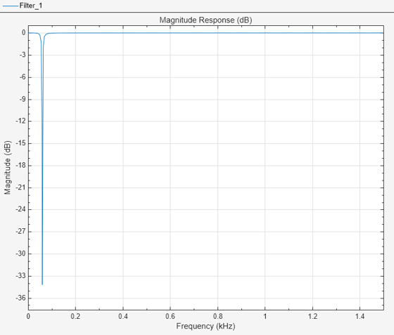
Suppose that you want to eliminate a 60 Hz interference in a signal sampled at 3000 Hz. You can use a second-order notch filter in this case and use the designNotchPeakIIR function to compute the coefficients of the filter. The function expects frequencies in normalized units. Scale the design parameters accordingly and specify them to the function. Use the Response="notch" option to design a notch filter and Response="peak" option to design a peak filter.
Fs = 3000;   % Sampling frequency is 3000 Hz
Fnyq = Fs/2; % Nyquist frequency is half the sampling frequency

F0 = 60;   % Interference is at 60 Hz
BW = 6;    % Choose a bandwidth factor of 6Hz
[num1,den1] = designNotchPeakIIR(Response="notch",CenterFrequency=F0/Fnyq,Bandwidth=BW/Fnyq,FilterOrder=2);
filterAnalyzer({num1,den1,1},SampleRates=Fs)

You can also design the filter by specifying the quality factor. Quality factor is defined as the ratio of the notch or peak frequency and the bandwidth : . The quality factor is a measure of how well you can isolate the desired frequency from the other frequencies. When you fix the filter order, you can achieve a higher by pushing the poles closer to the zeros. However, specifying the bandwidth is a more convenient way of achieving exactly the desired shape for the designed filter.
Design another second-order filter by specifying the quality factor and using it to calculate the 3-dB bandwidth. Use the designNotchPeakIIR function to compute the filter coefficients. Visualize the magnitude response of the filter.
Q2 = 100;    % Choose a Q factor of 100
[num2,den2] = designNotchPeakIIR(Response="notch",CenterFrequency=F0/Fnyq,QualityFactor=Q2,FilterOrder=2);
filterAnalyzer({num1,den1,1}, {num2,den2,1}, SampleRates=Fs, FilterNames=["notchQ10","notchQ100"])
Second-Order Peak Filters
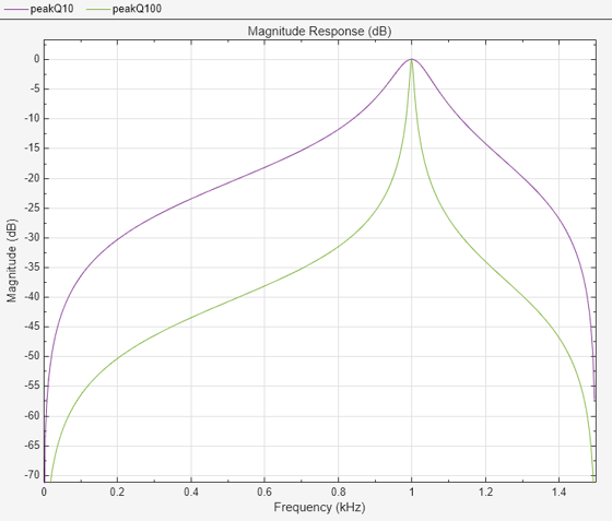
Peak filters are used to retain only a single frequency component (or a small band of frequencies) from a signal. Use the same designNotchPeakIIR function to compute the coefficients of a peak filter.
Fs = 3000;   % Sampling frequency is 3000 Hz
Fnyq = Fs/2; % Nyquist frequency is half the sampling frequency

F0 = 1000;   % Interference is at 60 Hz

Q1 = 10;
[num1, den1] = designNotchPeakIIR(Response="peak",CenterFrequency = F0/Fnyq,QualityFactor=Q1,FilterOrder=2);

Q2 = 100;
[num2, den2] = designNotchPeakIIR(Response="peak",CenterFrequency = F0/Fnyq,QualityFactor=Q2,FilterOrder=2);

filterAnalyzer({num1,den1,1}, {num2,den2,1}, SampleRates=Fs, FilterNames=["peakQ10","peakQ100"])

Time Varying Second-Order Notch Filter Implementation
Using time-varying filters requires changing the coefficients of the filter while the simulation runs. This is achieved by calling the designNotchPeakIIR function during runtime with the changing parameters. Alternatively, the DSP System Toolbox™ provides the dsp.NotchPeakFilter object to design and implement time-varying (tunable) second-order notch and peak filters.
Dynamic Simulation with Static Filter
In order to implement a time-varying filter, create a dynamic setup to simulate the filter and implement the filter with time-varying design parameters.
Start by creating a dynamic streamed simulation with filters whose coefficients do not change. Create two second-order notch filters, the first using the dsp.SOSFilter object and the second using the dsp.NotchFilter object. In the first filter, set the center frequency to 1 kHz, and the bandwidth at –3 dB to 500 Hz. Calculate the coefficients of this filter directly using the designNotchPeakIIR function. In the second filter, set the center frequency to 3 kHz and the bandwidth at –3 dB to 500 Hz. The sample rate for both filters is 8 kHz. Use the Verbose=true option to print the default values of unspecified parameters. In this case, FilterOrder is not specified and defaults to 2.
Fs = 8e3;    % 8 kHz sampling frequency
Fnyq = Fs/2; % Nyquist frequency

% Input parameters
samplesPerFrame = 256;
nFrames = 8192;

F01 = 1e3;   % Notch at 1 kHz for Filter 1
BW = 500;    % 500 Hz bandwidth for both filters
[b, a] = designNotchPeakIIR(Response="notch",CenterFrequency=F01/Fnyq,Bandwidth=BW/Fnyq,Verbose=true) % Filter 1 coefficients
designNotchPeakIIR(FilterOrder=2, CenterFrequency=0.25, Bandwidth=0.125, HasScaleValues=false, Response="notch", Datatype="double")
b = 1×3

    0.8341   -1.1796    0.8341
a = 1×3

    1.0000   -1.1796    0.6682
sosFilter = dsp.SOSFilter(b,a);

F02 = 3e3;    % Notch at 3 kHz for Filter 2

npFilter = dsp.NotchPeakFilter(CenterFrequency=F02,Bandwidth=BW,SampleRate=Fs);

scope = spectrumAnalyzer(PlotAsTwoSidedSpectrum=false, ...
    SampleRate=Fs, ...
    AveragingMethod="exponential",...
    ForgettingFactor=.95,...
    ChannelNames=["Filter 1","Filter 2"],...
    ShowLegend=true);

for k = 1:nFrames
   x = randn(samplesPerFrame, 1);
   y1 = sosFilter(x);
   y2 = npFilter(x);
   scope([y1,y2]);
end

Simulation with Time-Varying Filter
The coefficients of time-varying filters change over time due to runtime changes in the design parameters (for example, the center frequency for a notch filter). Create two second-order notch filters with time-varying design parameters. As with the static filter, use the designNotchPeakIIR function and the dsp.SOSFilter object to implement the first filter, and the dsp.NotchPeakFilter object to implement the second filter. Vary the design parameters of both filters over time.
% Notch filter parameters - how they vary over time
Fs = 8e3;                       % 8 kHz sampling frequency
F01 = 1e3 * [0.5, 1, 1.5, 3];   % Notch frequencies for Filter 1
F02 = 1e3 * [3.5, 3, 2.5, 2];   % Notch frequencies for Filter 2
BW = 500 * ones(1,4);           % 500 Hz bandwidth for both filters

myChangingParams1 = struct(f0=num2cell(F01/(Fs/2)),bw=num2cell(BW/(Fs/2)));
myChangingParams2 = struct(F0=num2cell(F02),BW=num2cell(BW));
paramsChangeTimes = [0, 70, 140, 210]; % in seconds

% Simulation time management
nSamplesPerFrame = 256;
tEnd = 300;
nSamples = ceil(tEnd * Fs);
nFrames = floor(nSamples / nSamplesPerFrame);

% Object creation
sosFilter = dsp.SOSFilter; %Filter 1 object
npFilter = dsp.NotchPeakFilter(SampleRate=Fs);
scope = spectrumAnalyzer(PlotAsTwoSidedSpectrum=false, ...
    SampleRate=Fs, ...
    AveragingMethod="exponential",...
    ForgettingFactor=.75,...
    ChannelNames=["Filter 1","Filter 2"],...
    ShowLegend=true);
paramtbl1 = ParameterTimeTable(Time=paramsChangeTimes, ...
    Values=myChangingParams1, ...
    SampleRate=Fs/nSamplesPerFrame);
paramtbl2 = ParameterTimeTable(Time=paramsChangeTimes, ...
    Values=myChangingParams2, ...
    SampleRate=Fs/nSamplesPerFrame);

% Actual simulation loop
for frameIdx = 1:nFrames
    % Get current F0 and BW
    [params1, update1] = paramtbl1();
    [params2, update2] = paramtbl2();
    if(update1)
        % Recompute filter coefficients if parameters changed
        [b, a] = designNotchPeakIIR(Response="notch",CenterFrequency=params1.f0,Bandwidth=params1.bw);
        % Set filter coefficients to new values
        sosFilter.Numerator = b;
        sosFilter.Denominator = a;
    end
    if(update2)
        npFilter.CenterFrequency = params2.F0;
        npFilter.Bandwidth = params2.BW;
    end
    % Generate vector of white noise samples
    x = randn(nSamplesPerFrame, 1);
    % Filter noise
    y1 = sosFilter(x);
    y2 = npFilter(x);
    % Visualize spectrum
    scope([y1,y2]);
end

You can implement a tunable peak filter similarly using the dsp.NotchPeakFilter object or by using the iirpeak function and dsp.SOSFilter object.
Note: The tunable peak and notch filters support code generation.
Higher Order Notch and Peak Filters
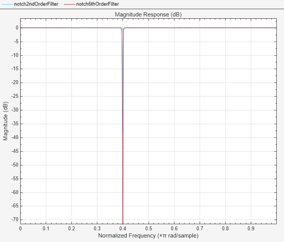
As you cannot push the poles beyond a point without affecting filter stability, in order to improve the brickwall approximation of the filter, you must increase the filter order. Use the FilterOrder design parameter to set the notch or peak filter order, and the SystemObject=true option to design a dsp.SOSFilter System object. Compare a second order notch filter design against a sixth order notch filter.
notchfilt2 = designNotchPeakIIR(Response="notch",FilterOrder=2,CenterFrequency=0.4,QualityFactor=100,SystemObject=true);
notchfilt6 = designNotchPeakIIR(Response="notch",FilterOrder=6,CenterFrequency=0.4,QualityFactor=100,SystemObject=true);

filterAnalyzer(notchfilt2, notchfilt6, FilterNames=["notch2ndOrderFilter","notch6thOrderFilter"])

Similarly, compare a second order peak filter design against an eighth order peak filter.
peakfilt2 = designNotchPeakIIR(Response="peak",FilterOrder=2,CenterFrequency=0.6,QualityFactor=80,SystemObject=true);
peakfilt8 = designNotchPeakIIR(Response="peak",FilterOrder=8,CenterFrequency=0.6,QualityFactor=80,SystemObject=true);

filterAnalyzer(peakfilt2, peakfilt8, FilterNames=["peak2ndOrderFilter", "peak8thOrderFilter"])
Higher Order Notch and Peak Filter with Passband and Stopband Ripple Control
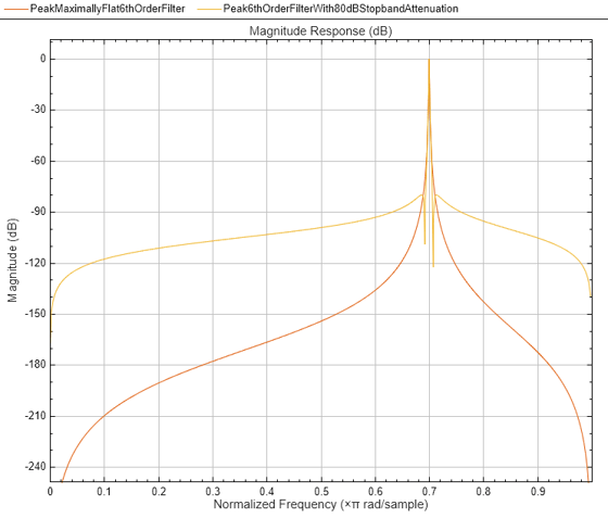
For a given filter order, you can obtain sharper transitions by allowing for passband or stopband ripples or both. This can be accomplished by using the "notchiir" and "peakiir" responses in designfilt. All specifications and tradeoffs mentioned so far apply equally to notch and peak filters.
N = 8; F0 = 0.4; BW = 0.1;
notchfilt = designNotchPeakIIR(Response="notch",FilterOrder=N,CenterFrequency=F0,Bandwidth=BW,SystemObject=true);
notchfilt1 = designfilt('notchiir',FilterOrder=N,CenterFrequency=F0,Bandwidth=BW,...
    PassbandRipple=0.5,StopbandAttenuation=60,SystemObject=true);

filterAnalyzer(notchfilt, notchfilt1, FilterNames=["NotchMaximallyFlat8thOrderFilter",...
    "Notch8thOrderFilterWithPassbandorStopbandRipples"])

N = 6;
F0 = 0.7;
BW = 0.001;
peakfilt = designNotchPeakIIR(Response="peak",FilterOrder=N,CenterFrequency=F0,Bandwidth=BW,SystemObject=true);
peakfilt1 = designfilt('peakiir',FilterOrder=N,CenterFrequency=F0,Bandwidth=BW,...
    StopbandAttenuation=80,SystemObject=true);
filterAnalyzer(peakfilt, peakfilt1, FilterNames=["PeakMaximallyFlat6thOrderFilter",...
    "Peak6thOrderFilterWith80dBStopbandAttenuation"])
