filter
Forward recursion of Bayesian nonlinear non-Gaussian state-space model
Since R2023b
Syntax
Description
filter estimates state-distribution moments of a
Bayesian nonlinear non-Gaussian state-space model (bnlssm), conditioned on model
parameters Θ, for each period of the specified response data by using importance sampling and
resampling in the sequential Monte Carlo (SMC) framework. filter
approximates the state filtering distribution and likelihood function by applying
particles, or weighted random samples.
[
returns approximate state-distribution means X,logL] = filter(Mdl,Y,params)X for each sampling time in
the input response data Y and the corresponding loglikelihood
logL resulting from performing forward recursion of, or filtering, the
Bayesian nonlinear state-space model Mdl.
filter evaluates the parameter map
Mdl.ParamMap by using the vector of parameter values
params.
filter filters Y and particles, weighted
random samples representing state values, through the model by using SMC.
[
additionally returns the following quantities using any of the input-argument combinations
in the previous syntaxes:X,logL,Output,RND] = filter(___)
Output— Filtering results by sampling periodApproximate loglikelihood values associated with the input data, input parameters, and particles
Filter estimate of state-distribution means
Filter estimate of state-distribution covariance
Custom statistics
Effective sample size
Flags indicating which data the software used to filter
Flags indicating resampling
RND— Normal random variables generated byfilterused to reproduce results or reuse random variates generated by a previous call offilter
Examples
This example uses simulated data to compute filter estimates of state distribution means of the following Bayesian nonlinear state-space model in equation. The state-space model contains two independent, stationary, autoregressive states each with a model constant. The observations are a nonlinear function of the states with Gaussian noise. The prior distribution of the parameters is flat. Symbolically, the system of equations is
and are the unconditional means of the corresponding states. The initial distribution moments of each state are their unconditional mean and covariance.
Create a Bayesian nonlinear state-space model characterized by the system. The observation equation is in equation form, that is, the function composing the states is nonlinear and the innovation series is additive, linear, and Gaussian. The Local Functions section contains two functions required to specify the Bayesian nonlinear state-space model: the state-space model parameter mapping function and the prior distribution of the parameters. You can use the functions only within this script.
Mdl = bnlssm(@paramMap,@priorDistribution)
Mdl =
  bnlssm with properties:

             ParamMap: @paramMap
    ParamDistribution: @priorDistribution
      ObservationForm: "equation"
           Multipoint: [1×0 string]
      ParticleOptions: [1×1 particleoptions]
Mdl is a bnlssm model specifying the state-space model structure and prior distribution of the state-space model parameters. Because Mdl contains unknown values, it serves as a template for posterior analysis with observations.
Simulate a series of 100 observations from the following stationary 2-D VAR process.
where the disturbance series are standard Gaussian random variables.
rng(1,"twister")    % For reproducibility
T = 100;
thetatrue = [0.9; 1; -0.75; -1; 0.3; 0.2; 0.1];
MdlSim = varm(AR={diag(thetatrue([1 3]))},Covariance=diag(thetatrue(5:6).^2), ...
    Constant=thetatrue([2 4]));
XSim = simulate(MdlSim,T);
Compose simulated observations using the following equation.
where the innovation series is a standard Gaussian random variable.
ysim = log(sum(exp(XSim - mean(XSim)),2)) + thetatrue(7)*randn(T,1);
To compute state estimates, the filter function requires response data and a model with known state-space model parameters. Choose a random set with the following constraints:
and are within the unit circle. Use to generate values.
and are real numbers. Use the distribution to generate values.
, , and are positive real numbers. Use the distribution to generate values.
theta13 = (-1+(1-(-1)).*rand(2,1));
theta24 = 3*randn(2,1);
theta567 = chi2rnd(1,3,1);
theta = [theta13(1); theta24(1); theta13(2); theta24(2); theta567];
Compute filtered state estimates and corresponding loglikelihood by passing the Bayesian nonlinear model, simulated data, and parameter values to filter.
[FilterX,logL] = filter(Mdl,ysim,theta);
size(FilterX)
ans = 1×2

   100     4
logL
logL =
-134.1053
FilterX is a 100-by-4 matrix of filter state estimates, with rows corresponding to periods in the sample and columns corresponding to the state variables. logL is the approximate loglikelihood function estimate evaluated at the data and parameter values.
Compare the loglikelihood logL and the loglikelihood computed using from the data simulation.
[FilterXSim,logLSim] = filter(Mdl,ysim,thetatrue);
logLSim
logLSim =
-0.4078
logLSim > logL, suggesting that the model evaluated at thetaSim has the better fit.
Plot the two sets of filter state estimates with the true state values.
figure
tiledlayout(2,1)
nexttile
plot([FilterX(:,1) FilterXSim(:,1) XSim(:,1)])
title("x_{t,1}")
legend("Filter State, random \theta","Filter State, true \theta","XSim")
nexttile
plot([FilterX(:,3) FilterXSim(:,3) XSim(:,2)])
title("x_{t,3}")
legend("Filter State, random \theta","Filter State, true \theta","XSim")

The filter state estimates using the true value of and the simulated state paths are close. The filter state estimates are far from the simulated state paths.
Local Functions
These functions specify the state-space model parameter mappings, in equation form, and log prior distribution of the parameters.
function [A,B,C,D,Mean0,Cov0,StateType] = paramMap(theta)
    A = @(x)blkdiag([theta(1) theta(2); 0 1],[theta(3) theta(4); 0 1])*x;
    B = [theta(5) 0; 0 0; 0 theta(6); 0 0];
    C = @(x)log(exp(x(1)-theta(2)/(1-theta(1))) + ...
        exp(x(3)-theta(4)/(1-theta(3))));
    D = theta(7);
    Mean0 = [theta(2)/(1-theta(1)); 1; theta(4)/(1-theta(3)); 1];
    Cov0 = diag([theta(5)^2/(1-theta(1)^2) 0 theta(6)^2/(1-theta(3)^2) 0]);
    StateType = [0; 1; 0; 1];     % Stationary state and constant 1 processes
end

function logprior = priorDistribution(theta)
    paramconstraints = [(abs(theta([1 3])) >= 1) (theta(5:7) <= 0)];
    if(sum(paramconstraints))
        logprior = -Inf;
    else
        logprior = 0;   % Prior density is proportional to 1 for all values
                        % in the parameter space.
    end
end
This example shows how to use filter and Bayesian optimization to calibrate a Bayesian nonlinear state-space. Consider this nonlinear state-space model.
where has a flat prior and the series and are standard Gaussian random variables.
Simulate Series
Simulate a series of 100 observations from the following stationary 2-D VAR process.
where the series and are standard Gaussian random variables.
rng(10,"twister")    % For reproducibility
T = 100;
thetaDGP = [0.5; 0.6; -1; 2; 0.75];
numparams = numel(thetaDGP);

MdlSim = arima(AR=thetaDGP(1),Variance=sqrt(thetaDGP(2)), ...
    Constant=0);
xsim = simulate(MdlSim,T);
ysim = exp(thetaDGP(3).*xsim) + thetaDGP(4) + thetaDGP(5)*randn(T,1);
Create Bayesian Nonlinear Model
Create a Bayesian nonlinear state-space model. The Local Functions section contains two functions required to specify the Bayesian nonlinear state-space model: the state-space model parameter mapping function and the prior distribution of the parameters. You can use the functions only within this script. Specify Multipoint=["A" "C"] because the state-transition and measurement-sensitivity parameter mappings in paraMap can evaluate multiple particles simultaneously.
Mdl = bnlssm(@paramMap,@priorDistribution,Multipoint=["A" "C"]);
Perform Random Exploration
One way to explore the parameter space for the point that maximizes the likelihood is by random exploration:
Randomly generated set of parameters.
Compute the loglikelihood for that set.
Repeat steps 1 and 2 many times.
Choose the set of parameters that yields the largest loglikelihood.
Perform random exploration for 500 epochs. Choose a random set using the following arbitrary recipe:
.
and are .
and are.
numepochs = 500;
numparticles = 10000;
theta = NaN(numparams,numepochs);
logL = NaN(numepochs,1);

for j = 1:numepochs
    theta(:,j) = [(-1+(1-(-1)).*rand(1,1)); chi2rnd(1,1,1); ...
        2*randn(2,1); chi2rnd(1,1,1);];
    [~,logL(j)] = filter(Mdl,ysim,theta(:,j),NumParticles=numparticles);
end
Choose the set of parameters that maximizes the loglikelihood.
[bestlogL,idx] = max(logL);
bestTheta = theta(:,idx);
[bestTheta thetaDGP]
ans = 5×2

    0.0073    0.5000
    0.1850    0.6000
    1.7649   -1.0000
    2.2315    2.0000
    0.9174    0.7500
The values that maximize the likelihood are fairly close to the values that generated the data.
Perform Bayesian Optimization
Bayesian optimization requires you to specify which variables require optimization and their support. To do this, use optimizableVariable to provide a name to the variable and its support. This example limits the support of each variable to a small interval; you must experiment with the support for your application.
thetaOp(5) = optimizableVariable("theta5",[0,2]);
thetaOp(1) = optimizableVariable("theta1",[0,0.9]);
thetaOp(2) = optimizableVariable("theta2",[0,2]);
thetaOp(3) = optimizableVariable("theta3",[-3,0]);
thetaOp(4) = optimizableVariable("theta4",[-3,3]);
thetaOp is an optimizableVariable object specifying the name and support of each variable of .
bayesopt accepts a function handle to the function that you want to minimize with respect to one argument and the optimizable variable specifications. Therefore, provide the function handle neglog, which is associated with the negative loglikelihood function filterneglogl located in Local Functions. Specify the Expected Improvement Plus acquisition function and an exploration ratio of 1.
neglogl = @(var)filterneglogl(var,Mdl,ysim,numparticles);

rng(1,"twister")
results = bayesopt(neglogl,thetaOp,AcquisitionFunctionName="expected-improvement-plus", ...
    ExplorationRatio=1);
|==================================================================================================================================================|
| Iter | Eval   | Objective   | Objective   | BestSoFar   | BestSoFar   |       theta1 |       theta2 |       theta3 |       theta4 |       theta5 |
|      | result |             | runtime     | (observed)  | (estim.)    |              |              |              |              |              |
|==================================================================================================================================================|
|    1 | Best   |      1025.7 |     0.14044 |      1025.7 |      1025.7 |       0.0761 |      0.51116 |     -0.78522 |       -2.272 |      0.44888 |
|    2 | Best   |      331.37 |    0.042512 |      331.37 |      371.87 |       0.5021 |       0.8957 |     -0.11662 |      -1.1518 |       1.8165 |
|    3 | Best   |      249.02 |     0.06091 |      249.02 |      249.05 |      0.67392 |      0.54178 |       -2.091 |     -0.82814 |      0.63451 |
|    4 | Accept |       382.2 |    0.056812 |      249.02 |      249.17 |      0.74179 |       1.8872 |      -1.9159 |      -2.5691 |        1.596 |
|    5 | Best   |      216.44 |    0.053895 |      216.44 |      216.43 |      0.61267 |      0.61924 |      -1.1149 |       2.9961 |      0.61643 |
|    6 | Best   |      164.22 |    0.029844 |      164.22 |      164.45 |      0.61401 |   0.00061238 |      -2.9589 |       1.8878 |       1.5293 |
|    7 | Accept |      360.44 |    0.066475 |      164.22 |      164.45 |      0.58377 |       1.9852 |      -2.9987 |     0.021019 |      0.77461 |
|    8 | Accept |      177.04 |    0.032601 |      164.22 |      164.72 |      0.89867 |    0.0018174 |      -1.0503 |       2.7783 |       1.8071 |
|    9 | Accept |      186.45 |    0.027238 |      164.22 |      164.84 |      0.80488 |    0.0084895 |     -0.01858 |       2.9768 |       1.0852 |
|   10 | Accept |      181.58 |    0.031654 |      164.22 |      170.57 |      0.63305 |     0.010143 |      -2.9852 |       2.8766 |       1.8758 |
|   11 | Accept |       45368 |     0.10667 |      164.22 |      165.11 |      0.89485 |     0.054412 |     -0.53673 |      -2.9919 |      0.11003 |
|   12 | Best   |      162.31 |    0.032938 |      162.31 |       162.6 |       0.2698 |      0.68563 |     -0.98857 |       2.0194 |       1.3013 |
|   13 | Accept |      359.73 |    0.062517 |      162.31 |      157.01 |       0.2811 |       0.9361 |      -0.9667 |      -2.9998 |      0.89534 |
|   14 | Accept |      263.37 |     0.05872 |      162.31 |      162.34 |      0.50983 |       1.5251 |      -1.4948 |      0.51053 |      0.16848 |
|   15 | Accept |      369.68 |    0.057789 |      162.31 |      157.65 |    0.0037925 |       1.9989 |      -1.0577 |      -2.9385 |       1.3728 |
|   16 | Accept |      229.22 |    0.039396 |      162.31 |      157.91 |     0.034141 |       1.1867 |    -0.065829 |       2.9967 |       0.8046 |
|   17 | Accept |      1715.4 |    0.050314 |      162.31 |      162.46 |      0.61096 |       1.7351 |     -0.78055 |       2.9987 |      0.12635 |
|   18 | Accept |      404.98 |    0.050681 |      162.31 |      159.96 |      0.65288 |        1.926 |      -2.0963 |        -2.98 |       1.3657 |
|   19 | Accept |      301.21 |    0.044498 |      162.31 |      161.42 |      0.53417 |        1.357 |       -1.871 |      -1.1603 |       1.9982 |
|   20 | Accept |      187.06 |      0.0254 |      162.31 |      161.72 |      0.48496 |       1.6999 |     -0.11741 |       2.9734 |       1.9948 |
|==================================================================================================================================================|
| Iter | Eval   | Objective   | Objective   | BestSoFar   | BestSoFar   |       theta1 |       theta2 |       theta3 |       theta4 |       theta5 |
|      | result |             | runtime     | (observed)  | (estim.)    |              |              |              |              |              |
|==================================================================================================================================================|
|   21 | Accept |      195.13 |    0.037314 |      162.31 |      162.59 |      0.14728 |       1.0093 |      -1.0169 |        1.304 |       1.9993 |
|   22 | Accept |       267.1 |    0.051942 |      162.31 |      160.31 |    0.0098611 |       1.4868 |      -2.9959 |       2.8978 |      0.43616 |
|   23 | Accept |       48902 |     0.08676 |      162.31 |      162.86 |      0.59476 |       0.2805 |      -2.1883 |        2.253 |      0.01358 |
|   24 | Accept |      306.62 |    0.055148 |      162.31 |      162.82 |      0.29311 |       1.9999 |      -2.1312 |      0.21527 |       1.0484 |
|   25 | Accept |      391.82 |    0.086634 |      162.31 |      169.13 |      0.62061 |       1.6603 |      -2.7799 |      -1.3096 |       0.2723 |
|   26 | Accept |      279.93 |    0.060962 |      162.31 |      162.19 |      0.22534 |       1.0983 |      -2.2553 |      0.30718 |      0.37723 |
|   27 | Best   |      157.86 |    0.041658 |      157.86 |      155.72 |      0.24103 |        1.397 |     -0.50905 |       1.8992 |       1.0484 |
|   28 | Accept |       335.6 |     0.05999 |      157.86 |       155.6 |      0.63559 |       1.9978 |      -1.0127 |      -2.8999 |       1.8455 |
|   29 | Accept |      228.85 |    0.029214 |      157.86 |      155.41 |      0.15199 |      0.46668 |     -0.40723 |      0.28012 |       1.5972 |
|   30 | Accept |      481.62 |    0.042412 |      157.86 |      154.52 |      0.21257 |      0.18003 |      -1.5181 |      -1.3322 |       1.2729 |

__________________________________________________________
Optimization completed.
MaxObjectiveEvaluations of 30 reached.
Total function evaluations: 30
Total elapsed time: 8.9831 seconds
Total objective function evaluation time: 1.6233

Best observed feasible point:
    theta1     theta2     theta3     theta4    theta5
    _______    ______    ________    ______    ______

    0.24103    1.397     -0.50905    1.8992    1.0484

Observed objective function value = 157.8586
Estimated objective function value = 154.5175
Function evaluation time = 0.041658

Best estimated feasible point (according to models):
    theta1     theta2     theta3     theta4    theta5
    _______    ______    ________    ______    ______

    0.24103    1.397     -0.50905    1.8992    1.0484

Estimated objective function value = 154.5175
Estimated function evaluation time = 0.041658
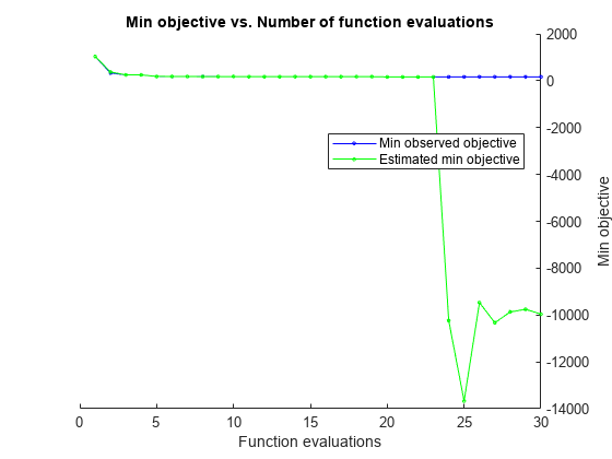
results is a BayesianOptmization object containing properties summarizing the results of Bayesian optimization.
Extract the value that minimizes the negative loglikelihood from results by using bestPoint.
bestPoint(results)
ans=1×5 table
    theta1     theta2     theta3     theta4    theta5
    _______    ______    ________    ______    ______

    0.24103    1.397     -0.50905    1.8992    1.0484
The results are fairly close to the values that generated the data.
Local Functions
These functions specify the state-space model parameter mappings, in equation form, and the log prior distribution of the parameters, and they compute the negative loglikelihood of the model.
function [A,B,C,D,Mean0,Cov0,StateType] = paramMap(theta)
    A = @(x)theta(1)*x;
    B = theta(2);
    C = @(x)exp(theta(3).*x) + theta(4);
    D = theta(5);
    Mean0 = 0;
    Cov0 = 1;
    StateType = 0;     % Stationary state process
end

function logprior = priorDistribution(theta)
    paramconstraints = [abs(theta(1)) >= 1; theta([2 4]) <= 0];
    if(sum(paramconstraints))
        logprior = -Inf;
    else
        logprior = 0;   % Prior density is proportional to 1 for all values
                        % in the parameter space.
    end
end

function neglogL = filterneglogl(theta,mdl,resp,np)
    theta = table2array(theta);
    [~,logL] = filter(mdl,resp,theta,NumParticles=np);
    neglogL = -logL;
end
When a set of state-space parameters are close in space, they can yield sufficiently different loglikelihood function values. This phenomenon is due to Monte Carlo sampling error. To address Monte Carlo sampling error so that comparisons among of loglikelihoods evaluated from similar parameter values during calibration is more fair, apply Hilbert sorting to the particles. This example reproduces results to show the effects of sorting particles.
Consider this simple linear Gaussian state-space model.
where the error series and are standard Gaussian random variables.
Assuming that the observation innovation variance is 1, simulate a response series of length 300 from the model. The Local Functions section contains the parameter mapping.
T = 300;
rng(1,"twister")    % For reproducibility
MdlTrue = ssm(@paramMap);
y = simulate(MdlTrue,T,Params=1);
Specify two values of , at which to evaluate the model, that are close to each other.
theta1 = 0.5;
theta2 = 0.5 + 1e-7;
Evaluate the true loglikelihood at each value of by using the filter function of ssm.
[~,logL1] = filter(MdlTrue,y,Params=theta1);
[~,logL2] = filter(MdlTrue,y,Params=theta2);
[logL1 logL2 abs(logL1-logL2)]
ans = 1×3

 -627.5987 -627.5987    0.0000
The values of yield practically identical loglikelihood values.
Create a Bayesian nonlinear state-space model using the parameter mapping and log prior density functions.
Mdl = bnlssm(@paramMap,@priorDistribution);
Evaluate the Bayesian loglikelihood at the values of .
[~,logL1] = filter(Mdl,y,theta1);
[~,logL2] = filter(Mdl,y,theta2);
[logL1 logL2 abs(logL1-logL2)]
ans = 1×3

 -629.1780 -628.4513    0.7267
Despite the arguments being close, there is a difference between their corresponding loglikelihoods. The difference can be attributed to Monte Carlo sampling.
Evaluate the loglikelihood at the value of again using the Bayesian model, but return the normal random variates to reproduce subsequent calls of filter.
[~,logL1,~,rnd] = filter(Mdl,y,theta1);
rnd
rnd = struct with fields:
    Autocorrelation: 1
               Time: 300
            Initial: [0×1000 double]
           Proposal: {300×1 cell}
           Resample: {300×1 cell}
       ResampleFlag: [300×1 logical]
rnd is a structure array containing sampling information.
Evaluate the loglikelihood at the value of again, but use the same normal random variates used to evaluate the loglikelihood at .
[~,logL2] = filter(Mdl,y,theta2,RND=rnd);
[logL1 logL2 abs(logL1-logL2)]
ans = 1×3

 -629.3398 -629.2906    0.0491
Still, the loglikelihoods are different.
Evaluate the loglikelihood at the values of by passing them and normal variates to filter again. Apply Hilbert sorting to the particles.
[~,logL1,~,rnd] = filter(Mdl,y,theta1,SortParticles=true);
[~,logL2] = filter(Mdl,y,theta2,RND=rnd,SortParticles=true);
[logL1 logL2 abs(logL1-logL2)]
ans = 1×3

 -631.4925 -631.4925    0.0000
Although the loglikelihood magnitudes are different from the frequentist state-space model, they are practically the same for values of that are very close to each other.
Local Functions
These functions specify the state-space model parameter mapping, in equation form, and log prior distribution of the parameter.
function [A,B,C,D,mean0,Cov0] = paramMap(theta)
    A = 1;
    B = 1;
    C = 1;
    D = theta;
    mean0 = 0;
    Cov0 = 0;
end

function logprior = priorDistribution(theta)
    paramconstraints = theta <= 0;
    if(sum(paramconstraints))
        logprior = -Inf;
    else
        logprior = 0;   % Prior density is proportional to 1 for all values
                        % in the parameter space.
    end
end
This example compares the performance of several SMC proposal particle resampling methods for obtaining filtered state estimates of a quasi-nonnegative constrained state space model, which models nonnegative state quantities such as interest rates and prices:
and are iid standard Gaussian random variables.
Generate Artificial Data
Consider the following data-generating process (DGP)
Generate a random series of 200 observations from the DGP.
a0 = 0.1;
a1 = 0.95;
b = 1;
d = 0.5;
theta = [a0; a1; b; d];
T = 50;

% Preallocate variables
x = zeros(T,1);
y = zeros(T,1);

rng(0,"twister") % For reproducibility
u = randn(T,1);
e = randn(T,1);

for t = 2:T
    x(t) = max(0,a0 + a1*x(t-1)) + b*u(t);
    y(t) = x(t) + d*e(t);
end
Create Bayesian Nonlinear State-Space Model
The Local Functions section contains two functions required to specify the Bayesian nonlinear state-space model: the state-space model parameter mapping function paramMap and the prior distribution of the parameters priorDistribution. You can use the functions only within this script.
The paramMap function has these qualities:
Functions can simultaneously evaluate the state equation for multiple values of
A. Therefore, you can speed up calculations by specifying theMultipoint="A"option.The observation equation is in equation form, that is, the function composing the states is nonlinear and the innovation series is additive, linear, and Gaussian.
The priorDistribution function specifies a flat prior, which has a density that is proportional to 1 everywhere in the parameter space; it constrains the error standard deviations to be positive.
Create a Bayesian nonlinear state-space model characterized by the system.
Mdl = bnlssm(@paramMap,@priorDistribution,Multipoint="A");Obtain Filtered State Estimates Using Each Proposal Sampler Method
Obtain filtered state estimates using the joint distribution of the parameters, at a randomly drawn set of values in [0,1], using the bootstrap, optimal, and one-pass unscented particle resampling methods. Specify drawing 5000 particles for SMC.
numParticles = 5000;
params = rand(4,1);
smcMethod = ["bootstrap" "optimal" "unscented"];
for j = 3:-1:1 % Set last element first to preallocate entire cell vector
    xFilter{j} = filter(Mdl,y,params,NewSamples=smcMethod(j),NumParticles=numParticles);
end
Compare the posterior means from each method with the true values.
figure
tiledlayout(3,1)
for j = 1:3
    nexttile
    plot([x xFilter{j}])
    title("SMC Method: " + upper(smcMethod(j)))
end
legend("True","Filter")
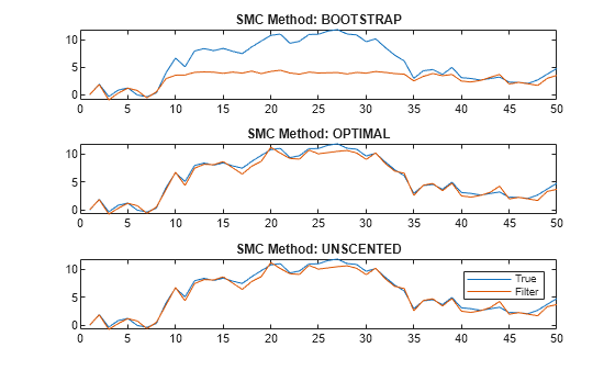
The figure shows that, in this case, the optimal and one-pass unscented methods yield filtered state estimates closer to the true values than the bootstrap method. For the bootstrap method, filtered state estimates in periods 10 through 35 level off around 5, while the true values jump as high as 10. The reason is the bootstrap filter updates particles solely by the transition equation—observations do not inform how particles are updated unlike the optimal and unscented methods.
Regardless of method, filter weighs particles by the observation densities. In this example, the observation equation is (as specified in params). For the bootstrap filter, the normally distributed observation innovation, with small loading 0.17, cannot accommodate large jumps, such as from 5 to 10. Consequently, the weights are degenerate: the largest particle takes all the weight, and filter discards the remaining particles during resampling because they have zero weight. The filtered states level off until period 35 when the observations fall below 5.
Local Functions
These functions specify the state-space model parameter mappings, in equation form, and log prior distribution of the parameters.
function [A,B,C,D,mean0,Cov0] = paramMap(params)
    a0 = params(1);
    a1 = params(2);
    b = params(3);
    d = params(4);
    A = @(x) max(0,a0+a1.*x);
    B = b;
    C = 1;
    D = d;
    mean0 = 0;
    Cov0 = 1;
end

function logprior = priorDistribution(theta)
    paramconstraints = theta(3:4) <= 0; % b and d are greater than 0
    if(sum(paramconstraints))
        logprior = -Inf;
    else
        logprior = 0;   % Prior density is proportional to 1 for all values
                        % in the parameter space.
    end
end
Input Arguments
Name-Value Arguments
Output Arguments
Tips
Smoothing has several advantages over filtering.
The smoothed state estimator is more accurate than the online filter state estimator because it is based on the full-sample data, rather than only observations up to the estimated sampling time.
A stable approximation to the gradient of the loglikelihood function, which is important for numerical optimization, is available from the smoothed state samples of the simulation smoother (finite differences of the approximated loglikelihood computed from the filter state estimates is numerically unstable).
You can use the simulation smoother to perform Bayesian estimation of the nonlinear state-space model via the Metropolis-within-Gibbs sampler.
Unless you set
Cutoff=0,filterresamples particles according to the specified resampling methodResample. Although resampling particles with high weights improves the results of the SMC, you should also allow the sampler traverse the proposal distribution to obtain novel, high-weight particles. To do this, experiment withCutoff.Avoid an arbitrary choice of the initial state distribution.
bnlssmfunctions generate the initial particles from the specified initial state distribution, which impacts the performance of the nonlinear filter. If the initial state specification is bad enough, importance weights concentrate on a small number of particles in the first SMC iteration, which might produce unreasonable filtering results. This vulnerability of the nonlinear model behavior contrasts with the stability of the Kalman filter for the linear model, in which the initial state distribution usually has little impact on the filter because the prior is washed out as it processes data.
Algorithms
filter accommodates missing data by not updating filtered state estimates corresponding to missing observations. In other words, suppose there is a missing observation at period t. Then, the state forecast for period t based on the previous t – 1 observations and filtered state for period t are equivalent.