Estimate Regression Model with ARMA Errors Using Econometric Modeler App
This example shows how to specify and estimate a regression model
with ARMA errors using the Econometric Modeler app. The data set, which is stored in
Data_USEconModel.mat, contains the US personal consumption
expenditures measured quarterly, among other series.
Consider modeling the US personal consumption expenditures
(PCEC, in $ billions) as a linear function of the effective
federal funds rate (FEDFUNDS), unemployment rate
(UNRATE), and real gross domestic product
(GDP, in $ billions with respect to the year 2000).
Import Data into Econometric Modeler
At the command line, load the Data_USEconModel.mat data
set.
load Data_USEconModelConvert the federal funds and unemployment rates from percents to decimals.
DataTimeTable.UNRATE = 0.01*DataTimeTable.UNRATE;
DataTimeTable.FEDFUNDS = 0.01*DataTimeTable.FEDFUNDS;
Convert the nominal GDP to real GDP by dividing all values by the GDP deflator
(GDPDEF) and scaling the result by 100. Create a column
in DataTimeTable for the real GDP series.
DataTimeTable.RealGDP = 100*DataTimeTable.GDP./DataTimeTable.GDPDEF;
At the command line, open the Econometric Modeler app.
econometricModeler
Alternatively, open the app from the apps gallery (see Econometric Modeler).
Import DataTimeTable into the app:
On the Modeler tab, in the Import section, click the Import button
 .
.In the Import Data dialog box, select the check box for the
DataTimeTablevariable.Click Import.
All time series variables in DataTimeTable appear in the
Time Series pane, and a time series plot of the series
appears in the Plot(COE) figure window.
Plot the Series
Plot the PCEC, RealGDP,
FEDFUNDS, and UNRATE
series on separate plots.
In the Time Series pane, double-click
PCEC.Repeat step 1 for
RealGDP,FEDFUNDS, andUNRATE.In the right pane, drag the Plot(PCEC) figure window to the top so that it occupies the first two quadrants.
Drag the Plot(RealGDP) figure window to the first quadrant.
Drag the Plot(UNRATE) figure window to the third quadrant.
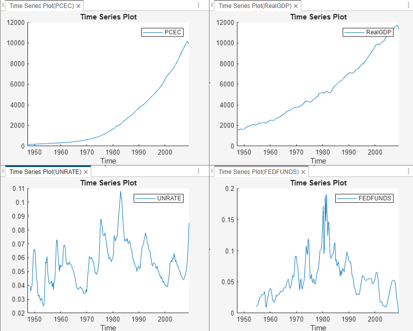
The PCEC and RealGDP
series appear to have an exponential trend. The
UNRATE and FEDFUNDS
series appear to have a stochastic trend.
Assess Collinearity Among Series
Check whether the series are collinear by performing Belsley collinearity diagnostics.
In the Time Series pane, select
PCEC. Then, press Ctrl and click to selectRealGDP,FEDFUNDS, andUNRATE.On the Modeler tab, in the Tests section, click Add Test > Belsley Collinearity Diagnostics.
The Belsley collinearity diagnostics results appear in the Collin(FEDFUNDS) document.
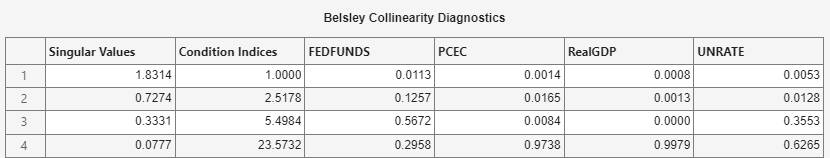
All condition indices are below the default condition-index tolerance, which is 30. The time series do not appear to be collinear.
Specify and Estimate Linear Model
Specify a linear model in which PCEC is the
response and RealGDP,
FEDFUNDS, and UNRATE
are predictors.
In the Time Series pane, select
PCEC.Click the Modeler tab. Then, in the Models section, click the arrow to display the models gallery.
In the models gallery, in the Regression Models section, click MLR.
In the MLR Model Parameters dialog box, in the Predictors section, clear the Include check box for the
COEtime series, and select the Include check box for theFEDFUNDS,RealGDP, andUNRATEtime series. Click Estimate.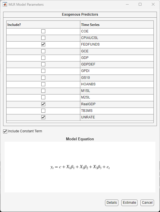
The model variable MLR_PCEC appears in the
Models pane, its value appears in the
Preview pane, and its estimation summary appears in the
Fit(MLR_PCEC) document.
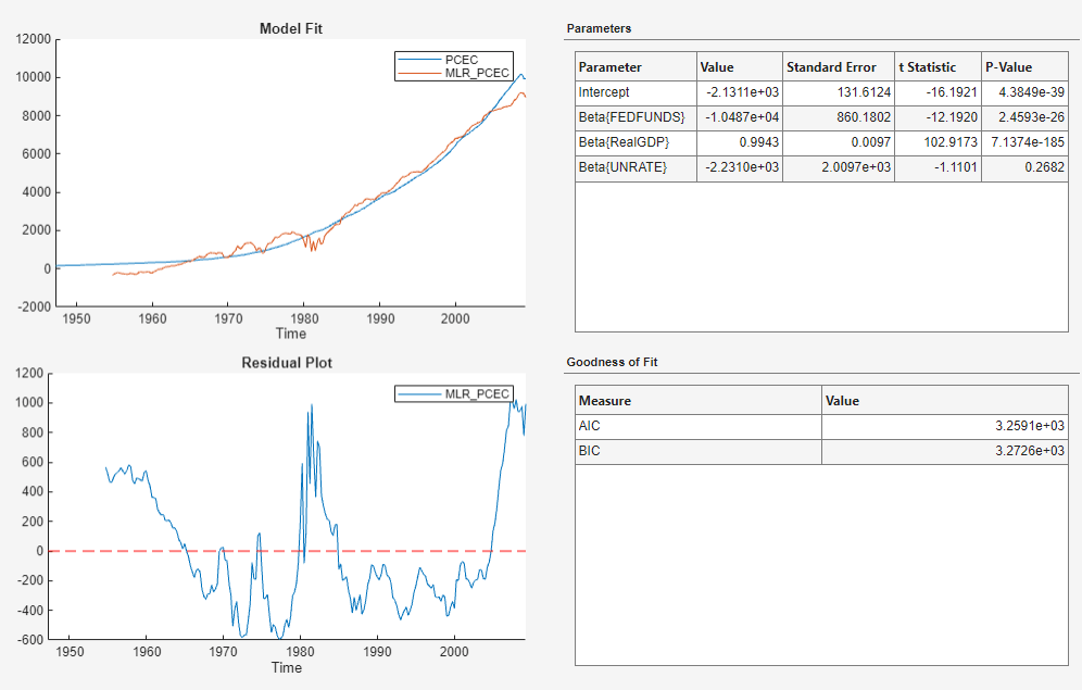
In the Fit(MLR_PCEC) figure window, the residual plot suggests that the standard linear model assumption of uncorrelated errors is violated. The residuals appear autocorrelated, nonstationary, and possibly heteroscedastic.
Stabilize Variables
To stabilize the residuals, stabilize the response and predictor series by
converting the PCEC and
RealGDP prices to returns, and by applying the
first difference to FEDFUNDS and
UNRATE.
Convert PCEC and RealGDP
prices to returns:
In the Time Series pane, select the
PCECtime series, then press Ctrl and select theRealGDPtime series.On the Modeler tab, in the Transforms section, click Log, then click Diff.
In the Time Series pane, variables representing the logged and differenced time series appear.
In the Time Series pane, rename the
PCEC_Log_DiffandRealGDP_Log_Diff. Click thePCEC_Log_Diffvariable twice to select its name and enterPCECReturns. Click theRealGDP_Log_Diffvariable twice to select its name and enterRealGDPReturns.
Apply the first difference to FEDFUNDS and
UNRATE:
In the Time Series pane, select the
FEDFUNDStime series, then press Ctrl and select theUNRATEtime series.On the Modeler tab, in the Transforms section, click Difference.
In the Time Series pane, variables representing the first difference of the time series appear.
Close all figure windows and documents.
Respecify and Estimate Linear Model
Respecify the linear model, but use the stabilized series instead.
In the Time Series pane, select
PCECReturns.On the Modeler tab, in the Models section, click the arrow to display the models gallery.
In the models gallery, in the Regression Models section, click MLR.
In the MLR Model Parameters dialog box, in the Predictors section, clear the Include check box for the
COEtime series, and select the Include check box for theFEDFUNDS_Diff,RealGDPReturns, andUNRATE_Difftime series. Click Estimate.
The model variable MLR_PCECReturns appears in the
Models pane, its value appears in the
Preview pane, and its estimation summary appears in the
Fit(MLR_PCECReturns) document.
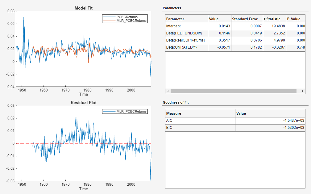
The residual plot suggests that the residuals are autocorrelated.
Check Goodness of Fit of Linear Model
Assess whether the residuals are normally distributed and autocorrelated by generating quantile-quantile and ACF plots.
Create a quantile-quantile plot of the
MLR_PCECReturns model residuals:
In the Time Series pane, select the
MLR_PCECReturnsmodel.On the Modeler tab, in the Diagnostics section, click Model Fit Diagnostics > Residual Q-Q Plot.
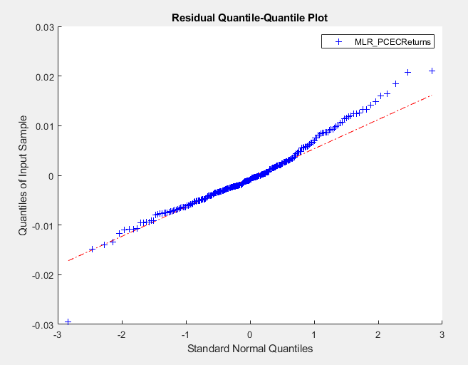
The residuals are skewed to the right.
Plot the ACF of the residuals:
In the Models pane, select the
MLR_PCECReturnsmodel.On the Modeler tab, in the Diagnostics section, click Model Fit Diagnostics > Residual Autocorrelation.
On the ACF tab, set Number of Lags to
40.
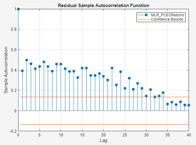
The plot shows autocorrelation in the first 34 lags.
Specify and Estimate Regression Model with ARMA Errors
Attempt to remedy the autocorrelation in the residuals by specifying a
regression model with ARMA(1,1) errors for
PCECReturns.
In the Time Series pane, select
PCECReturns.Click the Modeler tab. Then, in the Models section, click the arrow to display the models gallery.
In the models gallery, in the Regression Models section, click RegARMA.
In the regARMA Model Parameters dialog box:
In the Lag Order tab:
Set Autoregressive Order to
1.Set Moving Average Order to
1.
In the Predictors section, clear the Include check box for the
COEtime series, and select the Include check box for theFEDFUNDS_Diff,RealGDPReturns, andUNRATE_Difftime series.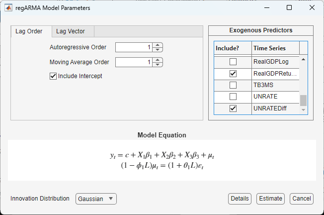
Click Estimate.
The model variable RegARMA_PCECReturns appears in
the Models pane, its value appears in the
Preview pane, and its estimation summary appears in the
Fit(RegARMA_PCECReturns) document.
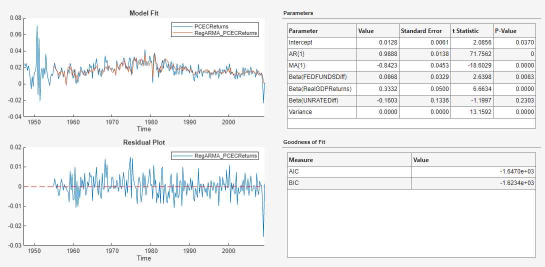
The t statistics suggest that all coefficients are
significant, except for the coefficient of
UNRATE_Diff. The residuals appear to fluctuate
around y = 0 without autocorrelation.
Check Goodness of Fit of ARMA Error Model
Assess whether the residuals of the
RegARMA_PCECReturns model are normally
distributed and autocorrelated by generating quantile-quantile and ACF
plots.
Create a quantile-quantile plot of the
RegARMA_PCECReturns model residuals:
In the Models pane, select the
RegARMA_PCECReturnsmodel.On the Modeler tab, in the Diagnostics section, click Model Fit Diagnostics > Residual Q-Q Plot.
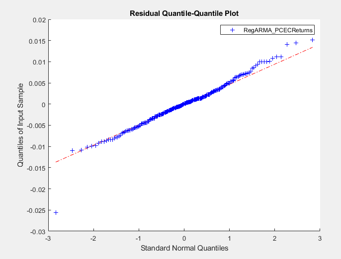
The residuals appear approximately normally distributed.
Plot the ACF of the residuals:
In the Models pane, select the
RegARMA_PCECReturnsmodel.On the Modeler tab, in the Diagnostics section, click Model Fit Diagnostics > Residual Autocorrelation.
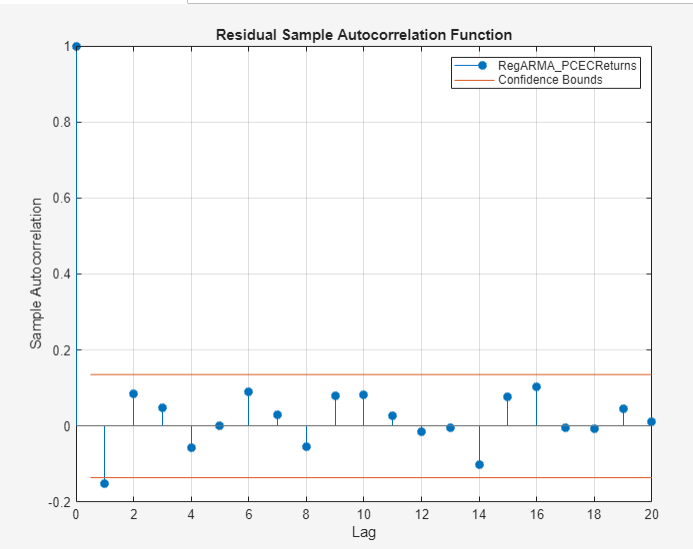
The first autocorrelation lag is significant.
From here, you can estimate multiple models that differ by the number of autoregressive and moving average polynomial orders in the ARMA error model. Then, choose the model with the lowest fit statistic. Or, you can check the predictive performance of the models by comparing forecasts to out-of-sample data.
See Also
Apps
Objects
Functions
estimate|fitlm|autocorr|collintest