Main Content

ecmnmle

Mean and covariance of incomplete multivariate normal data

Description

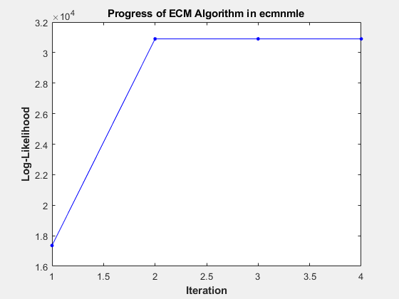
ecmnmle(Data) with no output arguments, this mode displays the convergence of the ECM algorithm in a plot by estimating objective function values for each iteration of the ECM algorithm until termination.

example

[Mean,Covariance] = ecmnmle(Data) estimates the mean and covariance of a data set (Data). If the data set has missing values, this routine implements the ECM algorithm of Meng and Rubin [2] with enhancements by Sexton and Swensen [3]. ECM stands for a conditional maximization form of the EM algorithm of Dempster, Laird, and Rubin [4].

example

[Mean,Covariance] = ecmnmle(___,InitMethod,MaxIterations,Tolerance,Mean0,Covar0) adds an optional arguments for InitMethod, MaxIterations, Tolerance,Mean0, and Covar0.

example

Examples

collapse all

This example shows how to compute the mean and covariance of incomplete multivariate normal data for five years of daily total return data for 12 computer technology stocks, with six hardware and six software companies

load ecmtechdemo.mat

The time period for this data extends from April 19, 2000 to April 18, 2005. The sixth stock in Assets is Google (GOOG), which started trading on August 19, 2004. So, all returns before August 20, 2004 are missing and represented as NaNs. Also, Amazon (AMZN) had a few days with missing values scattered throughout the past five years.

ecmnmle(Data)

Figure contains an axes object. The axes object with title Progress of ECM Algorithm in ecmnmle, xlabel Iteration, ylabel Log-Likelihood contains an object of type line.

ans = 12×1

    0.0008
    0.0008
   -0.0005
    0.0002
    0.0011
    0.0038
   -0.0003
   -0.0000
   -0.0003
   -0.0000
      ⋮

This plot shows that, even with almost 87% of the Google data being NaN values, the algorithm converges after only four iterations.

[Mean,Covariance] = ecmnmle(Data)
Mean = 12×1

    0.0008
    0.0008
   -0.0005
    0.0002
    0.0011
    0.0038
   -0.0003
   -0.0000
   -0.0003
   -0.0000
      ⋮

Covariance = 12×12

    0.0012    0.0005    0.0006    0.0005    0.0005    0.0003    0.0005    0.0003    0.0006    0.0003    0.0005    0.0006
    0.0005    0.0024    0.0007    0.0006    0.0010    0.0004    0.0005    0.0003    0.0006    0.0004    0.0006    0.0012
    0.0006    0.0007    0.0013    0.0007    0.0007    0.0003    0.0006    0.0004    0.0008    0.0005    0.0008    0.0008
    0.0005    0.0006    0.0007    0.0009    0.0006    0.0002    0.0005    0.0003    0.0007    0.0004    0.0005    0.0007
    0.0005    0.0010    0.0007    0.0006    0.0016    0.0006    0.0005    0.0003    0.0006    0.0004    0.0007    0.0011
    0.0003    0.0004    0.0003    0.0002    0.0006    0.0022    0.0001    0.0002    0.0002    0.0001    0.0003    0.0016
    0.0005    0.0005    0.0006    0.0005    0.0005    0.0001    0.0009    0.0003    0.0005    0.0004    0.0005    0.0006
    0.0003    0.0003    0.0004    0.0003    0.0003    0.0002    0.0003    0.0005    0.0004    0.0003    0.0004    0.0004
    0.0006    0.0006    0.0008    0.0007    0.0006    0.0002    0.0005    0.0004    0.0011    0.0005    0.0007    0.0007
    0.0003    0.0004    0.0005    0.0004    0.0004    0.0001    0.0004    0.0003    0.0005    0.0006    0.0004    0.0005
      ⋮

Input Arguments

collapse all

Data, specified as an NUMSAMPLES-by-NUMSERIES matrix with NUMSAMPLES samples of a NUMSERIES-dimensional random vector. Missing values are indicated by NaNs.

Data Types: double

(Optional) Initialization methods to compute the initial estimates for the mean and covariance of data, specified as a character vector. The initialization methods are:

  • 'nanskip' — Skip all records with NaNs.

  • 'twostage' — Estimate mean. Fill NaNs with the mean. Then estimate the covariance.

  • 'diagonal' — Form a diagonal covariance.

Note

If you supply Mean0 and Covar0, InitMethod is not executed.

Data Types: char

(Optional) Maximum number of iterations for the expectation conditional maximization (ECM) algorithm, specified as a numeric.

Data Types: double

(Optional) Convergence tolerance for the ECM algorithm, specified as a numeric. If Tolerance0, perform maximum iterations specified by MaxIterations and do not evaluate the objective function at each step unless in display mode.

Data Types: double

(Optional) Estimate for the mean, specified as an NUMSERIES-by-1 column vector. If you leave Mean0 unspecified ([]), the method specified by InitMethod is used. If you specify Mean0, you must also specify Covar0.

Data Types: double

(Optional) Estimate for the covariance, specified as an NUMSERIES-by-NUMSERIES matrix, where the input matrix must be positive-definite. If you leave Covar0 unspecified ([]), the method specified by InitMethod is used. If you specify Covar0, you must also specify Mean0.

Data Types: double

Output Arguments

collapse all

Maximum likelihood parameter estimates for the mean of the Data using ECM algorithm, returned as a NUMSERIES-by-1 column vector.

Maximum likelihood parameter estimates for the covariance of the Data using ECM algorithm, returned as a NUMSERIES-by-NUMSERIES matrix.

Algorithms

collapse all

Model

The general model is

ZN(Mean,Covariance),

where each row of Data is an observation of Z.

Each observation of Z is assumed to be iid (independent, identically distributed) multivariate normal, and missing values are assumed to be missing at random (MAR). See Little and Rubin [1] for a precise definition of MAR.

This routine estimates the mean and covariance from given data. If data values are missing, the routine implements the ECM algorithm of Meng and Rubin [2] with enhancements by Sexton and Swensen [3].

If a record is empty (every value in a sample is NaN), this routine ignores the record because it contributes no information. If such records exist in the data, the number of nonempty samples used in the estimation is ≤ NumSamples.

The estimate for the covariance is a biased maximum likelihood estimate (MLE). To convert to an unbiased estimate, multiply the covariance by Count/(Count – 1), where Count is the number of nonempty samples used in the estimation.

Requirements

This routine requires consistent values for NUMSAMPLES and NUMSERIES with NUMSAMPLES > NUMSERIES. It must have enough nonmissing values to converge. Finally, it must have a positive-definite covariance matrix. Although the references provide some necessary and sufficient conditions, general conditions for existence and uniqueness of solutions in the missing-data case, do not exist. The main failure mode is an ill-conditioned covariance matrix estimate. Nonetheless, this routine works for most cases that have less than 15% missing data (a typical upper bound for financial data).

Initialization Methods

This routine has three initialization methods that cover most cases, each with its advantages and disadvantages. The ECM algorithm always converges to a minimum of the observed negative log-likelihood function. If you override the initialization methods, you must ensure that the initial estimate for the covariance matrix is positive-definite.

The following is a guide to the supported initialization methods.

  • nanskip — The nanskip method works well with small problems (fewer than 10 series or with monotone missing data patterns). It skips over any records with NaNs and estimates initial values from complete-data records only. This initialization method tends to yield fastest convergence of the ECM algorithm. This routine switches to the twostage method if it determines that significant numbers of records contain NaN.

  • twostage — The twostage method is the best choice for large problems (more than 10 series). It estimates the mean for each series using all available data for each series. It then estimates the covariance matrix with missing values treated as equal to the mean rather than as NaNs. This initialization method is robust but tends to result in slower convergence of the ECM algorithm.

  • diagonal

    The diagonal method is a worst-case approach that deals with problematic data, such as disjoint series and excessive missing data (more than 33% of data missing). Of the three initialization methods, this method causes the slowest convergence of the ECM algorithm. If problems occur with this method, use display mode to examine convergence and modify either MaxIterations or Tolerance, or try alternative initial estimates with Mean0 and Covar0. If all else fails, try

    Mean0 = zeros(NumSeries);
    Covar0 = eye(NumSeries,NumSeries);
    

    Given estimates for mean and covariance from this routine, you can estimate standard errors with the companion routine ecmnstd.

Convergence

The ECM algorithm does not work for all patterns of missing values. Although it works in most cases, it can fail to converge if the covariance becomes singular. If this occurs, plots of the log-likelihood function tend to have a constant upward slope over many iterations as the log of the negative determinant of the covariance goes to zero. In some cases, the objective fails to converge due to machine precision errors. No general theory of missing data patterns exists to determine these cases. An example of a known failure occurs when two time series are proportional wherever both series contain nonmissing values.

References

[1] Little, Roderick J. A. and Donald B. Rubin. Statistical Analysis with Missing Data. 2nd Edition. John Wiley & Sons, Inc., 2002.

[2] Meng, Xiao-Li and Donald B. Rubin. “Maximum Likelihood Estimation via the ECM Algorithm.” Biometrika. Vol. 80, No. 2, 1993, pp. 267–278.

[3] Sexton, Joe and Anders Rygh Swensen. “ECM Algorithms that Converge at the Rate of EM.” Biometrika. Vol. 87, No. 3, 2000, pp. 651–662.

[4] Dempster, A. P., N. M. Laird, and Donald B. Rubin. “Maximum Likelihood from Incomplete Data via the EM Algorithm.” Journal of the Royal Statistical Society. Series B, Vol. 39, No. 1, 1977, pp. 1–37.

Version History

Introduced before R2006a