使用蒙特卡罗模拟进行对冲
此示例说明如何使用蒙特卡罗模拟来对一个过程产生不同结果的概率进行建模,该过程由于随机变量的介入而难以预测。
定义股票状况
假设某股票的设定如下。
% Price at time 0
Price_0 = 200;

% Drift (annualized)
Drift = 0.08;

% Volatility (annualized)
Vol = 0.4;

% Valuation date
Valuation = '01-Jan-2012';

% Investment horizon date
Horizon = '01-Jan-2013';

% Risk free rate
RiskFreeRate = 0.03;
使用蒙特卡罗模拟
模拟该股票从 Valuation 日到 Horizon 日的价格走势。
% Number of trials for the Monte Carlo simulation
NTRIALS = 100000;

% Length (in years) of the simulation
T = date2time(Valuation,Horizon,1,1);

% Number of periods per trial. Approximately 100 periods per year.
NPERIODS = round(100*T);

% Length (in years) of each time step per period
dt = T/NPERIODS;

% Instantiate the GBM object
StockGBM = gbm(Drift,Vol,'StartState',Price_0);

% Run the simulation
Paths = StockGBM.simByEuler(NPERIODS,'NTRIALS',NTRIALS, ...
    'DeltaTime',dt,'Antithetic',true);
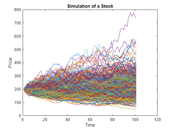
绘制股票模拟图
为了提高效率,仅绘制部分场景。
plot(squeeze(Paths(:,:,1:500)));
title('Simulation of a Stock');
xlabel('Time');
ylabel('Price');
使用布莱克-斯科尔斯模型计算股票的看跌期权
使用 blsprice 计算看跌期权。
Strike = 190;
[~,Put] = blsprice(Price_0,Strike,RiskFreeRate,T,Vol);
生成模拟矩阵
该模拟使用两种策略:(1) 仅持有股票,以及 (2) 持有股票并配以看跌期权对冲。
AssetScenarios = zeros(NTRIALS,2);
Price_T = squeeze(Paths(end,1,:));

% Strategy 1: Stock only
AssetScenarios(:,1) = (Price_T - Price_0) ./ Price_0
AssetScenarios = 100000×2
0.5927 0
-0.4069 0
-0.2526 0
0.3365 0
-0.3606 0
0.5549 0
-0.2211 0
0.3080 0
0.0849 0
-0.0416 0
0.1977 0
-0.1537 0
-0.1338 0
0.1681 0
-0.3236 0
⋮
% Strategy 2: Stock with put option cover
AssetScenarios(:, 2) = (max(Price_T, Strike) - (Price_0 + Put)) ./ ...
    (Price_0 + Put)
AssetScenarios = 100000×2

    0.5927    0.4266
   -0.4069   -0.1490
   -0.2526   -0.1490
    0.3365    0.1972
   -0.3606   -0.1490
    0.5549    0.3928
   -0.2211   -0.1490
    0.3080    0.1716
    0.0849   -0.0282
   -0.0416   -0.1415
    0.1977    0.0728
   -0.1537   -0.1490
   -0.1338   -0.1490
    0.1681    0.0463
   -0.3236   -0.1490
      ⋮
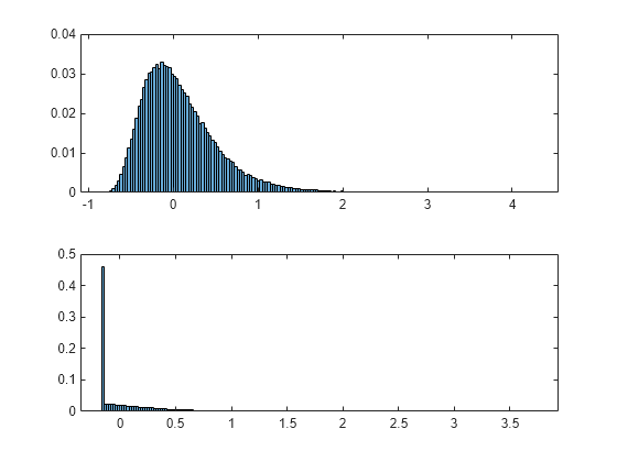
绘制分布图
这两种策略的收益均不遵循正态分布。
% Create histogram
figure;
subplot(2,1,1);
histogram(AssetScenarios(:,1),'Normalization','probability')
subplot(2,1,2);
histogram(AssetScenarios(:,2),'Normalization','probability')
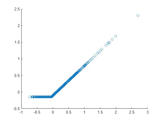
% Create scatter plot of the two strategies. Notice that the two strategies are highly
% correlated.
figure;
scatter(AssetScenarios(1:1000,1),AssetScenarios(1:1000,2));
创建 PortfolioCVaR 对象以获取投资组合权重
创建一个 PortfolioCVaR 对象。
p = PortfolioCVaR('Scenarios',AssetScenarios,'LowerBound',0, ...
    'Budget',1,'ProbabilityLevel',0.95)
p =
  PortfolioCVaR with properties:

                       BuyCost: []
                      SellCost: []
                  RiskFreeRate: []
              ProbabilityLevel: 0.9500
                      Turnover: []
                   BuyTurnover: []
                  SellTurnover: []
                  NumScenarios: 100000
                          Name: []
                     NumAssets: 2
                     AssetList: []
                      InitPort: []
                   AInequality: []
                   bInequality: []
                     AEquality: []
                     bEquality: []
                    LowerBound: [2×1 double]
                    UpperBound: []
                   LowerBudget: 1
                   UpperBudget: 1
                   GroupMatrix: []
                    LowerGroup: []
                    UpperGroup: []
                        GroupA: []
                        GroupB: []
                    LowerRatio: []
                    UpperRatio: []
                  MinNumAssets: []
                  MaxNumAssets: []
    ConditionalBudgetThreshold: []
        ConditionalUpperBudget: []
                     BoundType: []
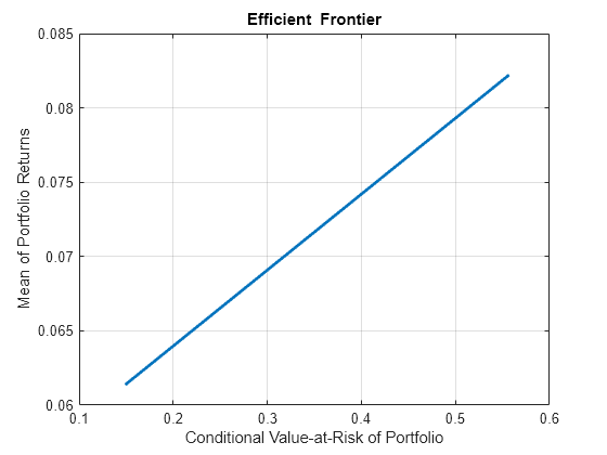
% Estimate the efficient frontier to obtain portfolio weights.
pwgt = estimateFrontier(p);

% Plot the efficient frontier.
figure;
plotFrontier(p,pwgt);
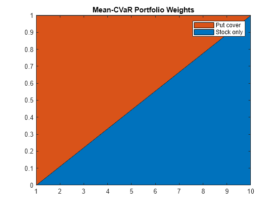
% Plot the portfolio weights.
figure;
area(pwgt');
axis([1 10 0 1])
legend('Stock only','Put cover');
title('Mean-CVaR Portfolio Weights');
添加对冲策略
使用 blsprice 计算不同行权价的看跌期权价格。
% Put option with strike at 50% of current underlying price
Strike50 = 0.50*Price_0;
[~, Put50] = blsprice(Price_0,Strike50,RiskFreeRate,T,Vol);

% Put option with strike at 75% of current underlying price
Strike75 = 0.75*Price_0;
[~, Put75] = blsprice(Price_0,Strike75,RiskFreeRate,T,Vol);

% Put option with strike at 90% of current underlying price
Strike90 = 0.90*Price_0;
[~, Put90] = blsprice(Price_0,Strike90,RiskFreeRate,T,Vol);

% Put option with strike at 95% of current underlying price
Strike95 = 0.95*Price_0; % Same as strike
[~, Put95] = blsprice(Price_0,Strike95,RiskFreeRate,T,Vol);
生成各策略的模拟矩阵
为不同的策略变体生成模拟矩阵。
AssetScenarios = zeros(NTRIALS, 5);

% Strategy 1: Stock only
AssetScenarios(:, 1) = (Price_T - Price_0) ./ Price_0;

% Strategy 2: Put option cover at 50%
AssetScenarios(:, 2) = (max(Price_T, Strike50) - (Price_0 + Put50)) ./ ...
    (Price_0 + Put50);

% Strategy 2: Put option cover at 75%
AssetScenarios(:, 3) = (max(Price_T, Strike75) - (Price_0 + Put75)) ./ ...
    (Price_0 + Put75);

% Strategy 2: Put option cover at 90%
AssetScenarios(:, 4) = (max(Price_T, Strike90) - (Price_0 + Put90)) ./ ...
    (Price_0 + Put90);

% Strategy 2: Put option cover at 95%
AssetScenarios(:, 5) = (max(Price_T, Strike95) - (Price_0 + Put95)) ./ ...
    (Price_0 + Put95);
使用对冲策略创建 PortfolioCVar 对象
使用对冲策略创建一个 PortfolioCVaR 对象。
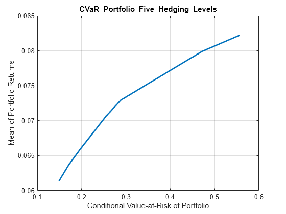
p = PortfolioCVaR('Name','CVaR Portfolio Five Hedging Levels', ...
   'AssetList',{'Stock','Hedge50','Hedge75','Hedge90','Hedge95'}, ...
   'Scenarios',AssetScenarios,'LowerBound',0, ...
   'Budget',1,'ProbabilityLevel',0.95);

% Estimate the efficient frontier to obtain portfolio weights.
pwgt = estimateFrontier(p);

% Plot the efficient frontier.
figure;
plotFrontier(p,pwgt);
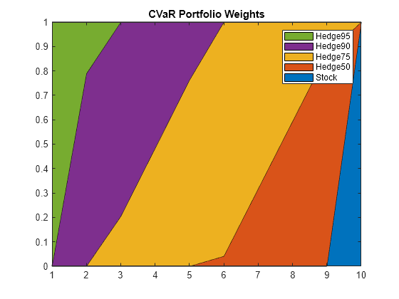
% Plot the portfolio weights.
figure;
area(pwgt');
legend(p.AssetList);
axis([1 10 0 1])
title('CVaR Portfolio Weights');
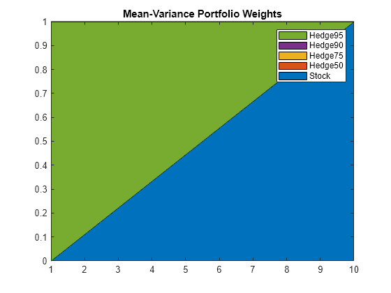
创建均值-方差投资组合
创建一个 Portfolio 对象,与 PortfolioCVaR 对象进行比较。
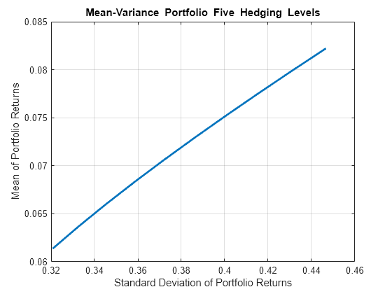
% Create the Portfolio object.
pmv = Portfolio('Name','Mean-Variance Portfolio Five Hedging Levels', ...
   'AssetList',{'Stock','Hedge50','Hedge75','Hedge90','Hedge95'});
pmv = pmv.estimateAssetMoments(p.getScenarios);
pmv = pmv.setDefaultConstraints;

% Estimate the efficient frontier to obtain portfolio weights.
pwgtmv = pmv.estimateFrontier;

% Plot the efficient frontier.
figure;
mvFrontierHandle = pmv.plotFrontier(pwgtmv);
% Plot the portfolio weights.
figure;
area(pwgtmv');
legend(pmv.AssetList);
axis([1 10 0 1])
title('Mean-Variance Portfolio Weights');
在均值-方差边界上绘制目标投资组合
确定可实现的收益水平。
% Achievable levels of return
pretlimits = pmv.estimatePortReturn(pmv.estimateFrontierLimits);
TargetRet = mean(pretlimits); % Target half way up the frontier

% Obtain risk level at target return
pwgtmvTarget = pmv.estimateFrontierByReturn(TargetRet);
priskTarget = pmv.estimatePortRisk(pwgtmvTarget);

% Plot point onto mean variance frontier
figure;
pmv.plotFrontier(pwgtmv);
hold on
scatter(priskTarget,TargetRet);
hold off

在 CVaR 边界上绘制均值-方差有效投资组合
下图显示目标投资组合位于均值-CVaR 有效边界之下。
% Obtain CVaR risk for mean variance target return portfolio
pretTargetCVaR = p.estimatePortReturn(pwgtmvTarget); % Should be TargetRet
priskTargetCVaR = p.estimatePortRisk(pwgtmvTarget);  % Risk proxy is CVaR

% Plot target return portfolio onto mean-CVaR frontier
figure;
p.plotFrontier(pwgt);
hold on
scatter(priskTargetCVaR,pretTargetCVaR);
hold off

另请参阅
主题
- Using Extreme Value Theory and Copulas to Evaluate Market Risk (Econometrics Toolbox)