poseplot

R2026b

3-D pose plot

collapse all in page

Syntax

poseplot

poseplot(orientation)

poseplot(___,position)

poseplot(___,frame)

poseplot(___,Name=Value)

poseplot(ax,___)

p = poseplot(___)

Description

The poseplot function plots a specified 3-D pose (position and orientation) as a patch with an xyz-frame at the patch origin. The poseplot function can plot a single or multiple 3-D poses.

poseplot plots the pose at the coordinate origin position with zero rotation. The default navigation frame is the north-east-down (NED) frame.

example

poseplot(orientation) plots the pose with the specified orientation. The position by default is [0 0 0]. To plot multiple poses, specify orientation as an array.

example

poseplot(___,position) specifies the position of the pose plot. To plot multiple poses, specify position as a matrix.

example

poseplot(___,frame) specifies the navigation frame of the pose plot.

poseplot(___,Name=Value) specifies pose patch properties using one or more name-value arguments. The properties apply to all the plotted poses. For example, poseplot(FaceColor="r") plots the pose with red face color. For a list of properties, see PosePatch Properties.

example

poseplot(ax,___) specifies the parent axes of the pose plot.

p = poseplot(___) returns a PosePatch object or an array of PosePatch objects. Use p to modify properties of the pose plot after creation. For a list of properties, see PosePatch Properties.

example

Examples

collapse all

Visualize Pose Using `poseplot`

Open Live Script

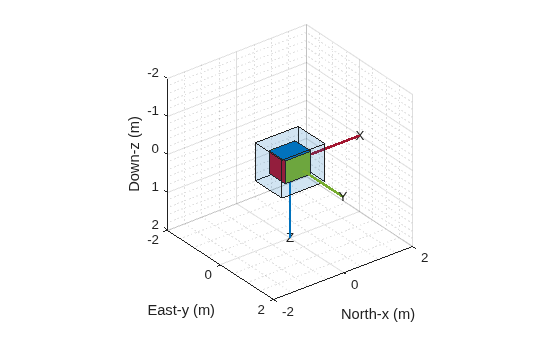
Plot the default pose using the poseplot function with default settings.

poseplot
xlabel("North-x (m)")
ylabel("East-y (m)")
zlabel("Down-z (m)");

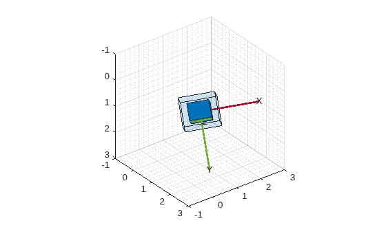
Figure contains an axes object. The axes object with xlabel North-x (m), ylabel East-y (m) is empty.

Next, plot a pose with specified orientation and position.

q = quaternion([35 10 50],"eulerd","ZYX","frame");
position = [1 1 1];
poseplot(q,position)

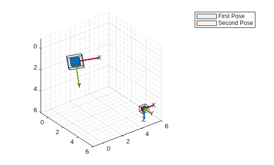
Figure contains an axes object. The axes object is empty.

Then, plot a second pose on the figure and return the PosePatch object. Plot the second pose with a smaller size by using the ScaleFactor name-value argument.

hold on
p = poseplot(eye(3),[5 5 5],ScaleFactor=0.5)

p = 
  PosePatch with properties:

    Orientation: [3×3 double]
       Position: [5 5 5]

  Show all properties

legend("First Pose","Second Pose")
hold off

Figure contains an axes object. The axes object is empty. These objects represent First Pose, Second Pose.

Animate Pose Using `poseplot`

Open Live Script

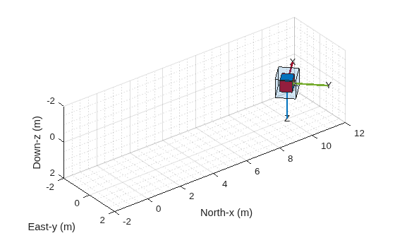
Animate a series of poses using the poseplot function. First, define the initial and final positions.

ps = [0 0 0];
pf = [10 0 0];

Then, define the initial and final orientations using the quaternion object.

qs = quaternion([45,0,0],'eulerd','ZYX','frame');
qf = quaternion([-45,0,0],'eulerd','ZYX','frame');

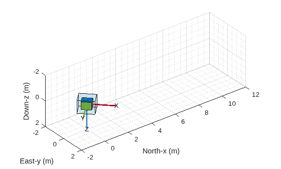
Show the starting pose.

patch = poseplot(qs,ps);
ylim([-2 2])
xlim([-2 12])
xlabel("North-x (m)")
ylabel("East-y (m)")
zlabel("Down-z (m)");

Figure contains an axes object. The axes object with xlabel North-x (m), ylabel East-y (m) is empty.

Change the position and orientation continuously using coefficients, and update the pose using the set object function.

for coeff = 0:0.01:1
    q = slerp(qs,qf,coeff);
    position = ps + (pf - ps)*coeff;
    set(patch,Orientation=q,Position=position); 
    drawnow
end

Figure contains an axes object. The axes object with xlabel North-x (m), ylabel East-y (m) is empty.

Reduce Clutter When Plotting Multiple Poses

Open Live Script

Plot multiple poses in a single call to the poseplot function, then hide the pose axis labels and origin boxes to reduce visual clutter.

Define 10 poses along a spiral trajectory. Create a 10-by-3 matrix of positions and a 10-by-1 array of quaternion orientations that rotate to follow the path.

numPoses = 10;
t = linspace(0,2*pi,numPoses)';
positions = [5*cos(t),5*sin(t),2*t];
orientations = quaternion([t+pi/2,zeros(numPoses,1),zeros(numPoses,1)],"euler","ZYX","frame");

Plot all 10 poses in a single call. By default, the poseplot function draws an origin box and pose axis labels at every pose, which can make a plot of many poses look cluttered.

figure
p1 = poseplot(orientations,positions);
axis equal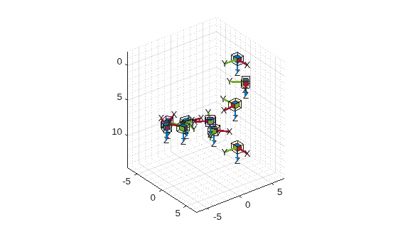

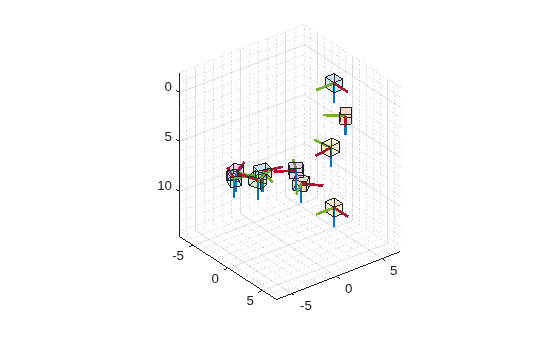
Figure contains an axes object. The axes object is empty.

Reduce the clutter by hiding the pose axis labels and origin boxes. Set the PoseAxisLabels and OriginBox properties to "off". Plot the poses in a new figure to compare the result with the previous plot.

figure
p2 = poseplot(orientations,positions,PoseAxisLabels="off",OriginBox="off");
axis equal

Figure contains an axes object. The axes object is empty.

Show Poses with Meshes

Open Live Script

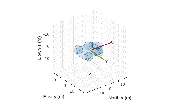
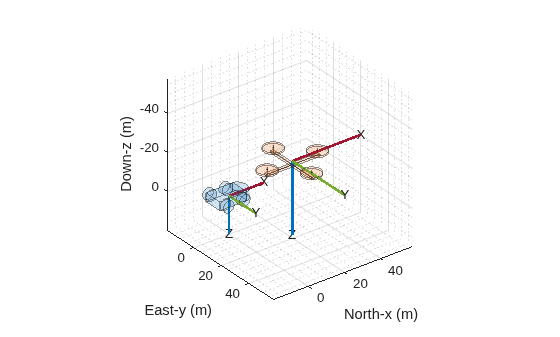
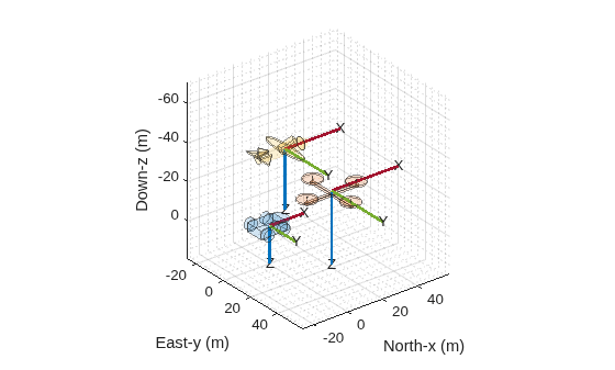
Plot orientations and positions in meshes using the poseplot function. First, plot a ground vehicle at the origin with zero rotation.

poseplot(ones("quaternion"),[0 0 0],MeshFileName="groundvehicle.stl",ScaleFactor=0.3);
xlabel("North-x (m)")
ylabel("East-y (m)")
zlabel("Down-z (m)")

Figure contains an axes object. The axes object with xlabel North-x (m), ylabel East-y (m) is empty.

Second, plot a rotor at the position [20 20 -20] with zero rotation.

hold on
poseplot(ones("quaternion"),[20 20 -20],MeshFileName="multirotor.stl",ScaleFactor=0.2);

Figure contains an axes object. The axes object with xlabel North-x (m), ylabel East-y (m) is empty.

Lastly, plot a fixed-wing aircraft at the position [5 5 -40] with zero rotation.

poseplot(ones("quaternion"),[5 5 -40],MeshFileName="fixedwing.stl",ScaleFactor=0.4);
view([-37.8 28.4])
hold off

Figure contains an axes object. The axes object with xlabel North-x (m), ylabel East-y (m) is empty.

Input Arguments

collapse all

`orientation` — Orientation
`quaternion(1,0,0,0)` (default) | `quaternion` object | 3-by-3 orthonormal matrix | N-element array of `quaternion` objects | 3-by-3-by-N array of 3-by-3 orthonormal matrices

Orientation, specified as a quaternion object, a 3-by-3 orthonormal rotation matrix, an array of quaternion objects, or a 3-by-3-by-N array of orthonormal matrices. To plot multiple poses in a single function call, specify orientation as an N-element array of quaternion objects or a 3-by-3-by-N array of orthonormal rotation matrices, where N is the number of poses. Each 3-by-3 page of the 3-by-3-by-N array is the orthonormal rotation matrix for the corresponding pose.

Note

A 3-by-3 matrix input is always interpreted as a single rotation matrix, not as three positions.

If you specify one orientation and N positions, poseplot expands the single orientation N times and plots N poses.

If you specify more than one orientation and more than one position, the number of orientations and positions must be equal. Otherwise, an error occurs during plotting.

Example: quaternion([pi/2 0 pi/4],"euler","ZYX","frame")

Example: eul2rotm([pi/2 0 pi/4],"ZYX")

`position` — Position of pose plot
`[0 0 0]` (default) | three-element real-valued vector | N-by-3 matrix

Position of the pose plot, specified as a three-element real-valued vector or N-by-3 matrix. To plot multiple poses, specify an N-by-3 matrix, where N is the number of poses and each row is the position for the corresponding pose.

Note

A 3-by-3 matrix input is always interpreted as a single rotation matrix, not as three positions.

If you specify one position and N rotations, poseplot expands the single position N times and plots N poses.

If you specify more than one position and more than one rotation, the number of positions and rotations must be equal. Otherwise, an error occurs during plotting.

Example: [1 3 4]

`frame` — Navigation frame of pose plot
`"NED"` (default) | `"ENU"`

Navigation frame of the pose plot, specified as "NED" for the north-east-down frame or "ENU" for the east-north-up frame.

When the parent axes status is hold off, specifying the NED navigation frame reverses the y- and z-axes in the figure by setting the YDir and ZDir properties of the parent axes.

`ax` — Parent axes of pose plot
`Axes` object

Parent axes of the pose plot, specified as an Axes object. If you do not specify the axes, the poseplot function uses the current axes.

Name-Value Arguments

collapse all

Specify optional pairs of arguments as Name1=Value1,...,NameN=ValueN, where Name is the argument name and Value is the corresponding value. Name-value arguments must appear after other arguments, but the order of the pairs does not matter.

Example: poseplot(FaceAlpha=0.1)

The PosePatch properties listed here are only a subset. For a complete list, see PosePatch Properties.

`Orientation` — Orientation of pose plot
`quaternion(1,0,0,0)` object (default) | rotation matrix

Orientation of the pose plot, specified as a quaternion object or a rotation matrix.

`Position` — Position of pose plot
`[0 0 0]` (default) | three-element real-valued vector

Position of the pose plot, specified as a three-element real-valued vector.

`MeshFileName` — Name of STL mesh file
string scalar | character vector

This property is read-only after object creation.

Name of Standard Triangle Language (STL) mesh file, specified as a string scalar or a character vector containing the name of the mesh file. When you specify this argument, the poseplot function plots the mesh instead of the orientation box.

`ScaleFactor` — Scale factor of pose plot
`1` (default) | nonnegative scalar

Scale factor of the pose plot, specified as a nonnegative scalar. The scale factor controls the size of the orientation box. When you specify the MeshFileName argument, the scale factor also changes the scale of the mesh.

`FaceColor` — Face color of pose patch
RGB triplet | hexadecimal color code | `"r"` | `"g"` | `"b"` | ...

Face color of pose patch, specified as an RGB triplet, a hexadecimal color code, a color name, or a short name.

An RGB triplet is a three-element row vector whose elements specify the intensities of the red, green, and blue components of the color. The intensities must be in the range [0, 1]; for example, [0.4 0.6 0.7].
A hexadecimal color code is a character vector or a string scalar that starts with a hash symbol (#) followed by three or six hexadecimal digits, which can range from 0 to F. The values are not case sensitive. Thus, the color codes "#FF8800", "#ff8800", "#F80", and "#f80" are equivalent.

The default value is an RGB triplet from the ColorOrder property of the axes. The SeriesIndex property of the PosePatch object determines which color from the ColorOrder the pose plot uses.

Here is a list of commonly used colors and their corresponding values.

Color Name	Short Name	RGB Triplet	Hexadecimal Color Code
`"red"`	`"r"`	`[1 0 0]`	`"#FF0000"`
`"green"`	`"g"`	`[0 1 0]`	`"#00FF00"`
`"blue"`	`"b"`	`[0 0 1]`	`"#0000FF"`
`"cyan"`	`"c"`	`[0 1 1]`	`"#00FFFF"`
`"magenta"`	`"m"`	`[1 0 1]`	`"#FF00FF"`
`"yellow"`	`"y"`	`[1 1 0]`	`"#FFFF00"`
`"black"`	`"k"`	`[0 0 0]`	`"#000000"`
`"white"`	`"w"`	`[1 1 1]`	`"#FFFFFF"`

`FaceAlpha` — Face transparency of pose patch
`0.1` (default) | scalar in range `[0, 1]`

Face transparency of pose patch, specified as a scalar in range [0, 1]. A value of 1 is fully opaque and 0 is completely transparent.

`EdgeDensity` — Edge density of mesh
`0.8` (default) | numeric scalar in range `[0, 1]`

Since R2026b

This property is read-only after object creation.

Edge density of mesh, specified as a numeric scalar in the range [0, 1]. This property controls the density of edges displayed on a mesh specified by MeshFileName.

A value of 0 hides all edges. A value of 1 displays all edges. Between 0 and 1, higher values display more edges.

Setting this property has no effect if you do not specify MeshFileName.

For more information about EdgeDensity, see the More About section.

Data Types: single | double

`OriginBox` — Visibility of origin box
`"on"` (default) | `"off"` | on/off logical value

Since R2026b

Visibility of the origin box, specified as "on" or "off", or as numeric or logical 1 (true) or 0 (false). A value of "on" is equivalent to true, and "off" is equivalent to false. Thus, you can use the value of this property as a logical value. The value is stored as an on/off logical value of type matlab.lang.OnOffSwitchState.

"on" — Display the box at the origin of the pose.
"off" — Hide the origin box. Use this option to improve plot visibility when displaying a large number of poses simultaneously.

Setting this property has no effect when you specify a mesh using MeshFileName. Specifying MeshFileName hides the origin box.

`PoseAxisLabels` — Visibility of pose axis labels
`"on"` (default) | `"off"` | on/off logical value

Since R2026b

Visibility of pose axis labels, specified as "on" or "off", or as numeric or logical 1 (true) or 0 (false). A value of "on" is equivalent to true, and "off" is equivalent to false. Thus, you can use the value of this property as a logical value. The value is stored as an on/off logical value of type matlab.lang.OnOffSwitchState.

"on" — Display the X, Y, and Z axis labels at the tips of the pose axes.
"off" — Hide the axis labels. Use this option to improve plot visibility when displaying a large number of poses simultaneously.

Output Arguments

collapse all

`p` — Pose patch object
`PosePatch` object | N-by-1 array of `PosePatch` objects

Pose patch object, returned as a PosePatch object or N-by-1 array of PosePatch objects. When you plot multiple poses, poseplot returns an N-by-1 array of PosePatch objects. You can use the returned object to query and modify properties of the plotted pose. For a list of properties, see PosePatch Properties.

More About

collapse all

EdgeDensity

The EdgeDensity value determines the filter angle used to identify the edges to be displayed. The filter angle in radians is (1 - EdgeDensity) × π. An edge is displayed when the dihedral angle between its two adjacent triangular faces deviates from π radians by more than the filter angle. For more information on filter angle, see the featureEdges documentation.

Version History

Introduced in R2021b

expand all

R2026b: Plot multiple poses with improved performance

You can now plot multiple poses in a single poseplot function call by specifying multiple orientations to the orientation input argument and specifying multiple positions to the position input argument.

Using a single function call makes your code more concise and delivers performance improvements for workflows involving trajectories or time-series pose estimates. For example, the code below plots 1000 poses. In R2026a, you do this using a loop, whereas in R2026b, you can use array inputs. The R2026b code using arrays is about 5x faster:

R2026a:

function timingTest
    numPoses = 1000;
    orientations = quaternion(randn(numPoses,4));
    positions = cumsum(randn(numPoses,3), 1);
    
    for i = 1:numPoses
        poseplot(orientations(i), positions(i,:), 'ENU', MeshFileName = 'multirotor.stl');
    end
end

R2026b:

function timingTest
    numPoses = 1000;
    orientations = quaternion(randn(numPoses,4));
    positions = cumsum(randn(numPoses,3), 1);
    
    poseplot(orientations, positions, 'ENU', MeshFileName = 'multirotor.stl');
end

The approximate execution times are:

R2026a: 45.34 s
R2026b: 9.87 s

The code was timed on a Windows^® 11, AMD Epyc® 74F3 24-Core Processor CPU @ 3.19 GHz test system using the timeit function:

timeit(@timingTest)

R2026b: Control visibility of origin box and pose axis labels

You can now control the visibility of the origin box and pose axis labels of a pose using the new OriginBox and PoseAxisLabels properties of PosePatch Properties, respectively. You can use these properties to improve plot readability when displaying a large number of poses simultaneously.

R2026b: Control display of mesh edges

You can now control the density of mesh edges displayed using the new EdgeDensity property of PosePatch. You can also control the color, transparency, and width of edges using the new EdgeColor, EdgeAlpha, and EdgeLineWidth properties of PosePatch, respectively.

R2026b: Default display of mesh edges changed

Starting in R2026b, when you specify an STL mesh using the MeshFileName argument, poseplot displays only edges whose adjacent faces meet at a dihedral angle that deviates from 180 degrees by more than (1 - EdgeDensity) × 180 degrees. With the default EdgeDensity value of 0.8, only edges sharper than 36 degrees are shown by default. In previous releases, all mesh edges were displayed by default.

To use the previous default behavior, set EdgeDensity to 1:

poseplot(MeshFileName="groundvehicle.stl",EdgeDensity=1)

R2026b: `PatchFaceColor` and `PatchFaceAlpha` properties renamed

The PatchFaceColor and PatchFaceAlpha properties of PosePatch are now called FaceColor and FaceAlpha, respectively. The behavior of both properties remains the same. There are no plans to remove support for existing references to PatchFaceColor and PatchFaceAlpha.

poseplot

Syntax

Description

Examples

Visualize Pose Using poseplot

Animate Pose Using poseplot

Reduce Clutter When Plotting Multiple Poses

Show Poses with Meshes

Input Arguments

orientation — Orientation quaternion(1,0,0,0) (default) | quaternion object | 3-by-3 orthonormal matrix | N-element array of quaternion objects | 3-by-3-by-N array of 3-by-3 orthonormal matrices

position — Position of pose plot [0 0 0] (default) | three-element real-valued vector | N-by-3 matrix

frame — Navigation frame of pose plot "NED" (default) | "ENU"

ax — Parent axes of pose plot Axes object

Name-Value Arguments

Orientation — Orientation of pose plot quaternion(1,0,0,0) object (default) | rotation matrix

Position — Position of pose plot [0 0 0] (default) | three-element real-valued vector

MeshFileName — Name of STL mesh file string scalar | character vector

ScaleFactor — Scale factor of pose plot 1 (default) | nonnegative scalar

FaceColor — Face color of pose patch RGB triplet | hexadecimal color code | "r" | "g" | "b" | ...

FaceAlpha — Face transparency of pose patch 0.1 (default) | scalar in range [0, 1]

EdgeDensity — Edge density of mesh 0.8 (default) | numeric scalar in range [0, 1]

OriginBox — Visibility of origin box "on" (default) | "off" | on/off logical value

PoseAxisLabels — Visibility of pose axis labels "on" (default) | "off" | on/off logical value

Output Arguments

p — Pose patch object PosePatch object | N-by-1 array of PosePatch objects

More About

EdgeDensity

Version History

R2026b: Plot multiple poses with improved performance

R2026b: Control visibility of origin box and pose axis labels

R2026b: Control display of mesh edges

R2026b: Default display of mesh edges changed

R2026b: PatchFaceColor and PatchFaceAlpha properties renamed

See Also

Visualize Pose Using `poseplot`

Animate Pose Using `poseplot`

`orientation` — Orientation
`quaternion(1,0,0,0)` (default) | `quaternion` object | 3-by-3 orthonormal matrix | N-element array of `quaternion` objects | 3-by-3-by-N array of 3-by-3 orthonormal matrices

`position` — Position of pose plot
`[0 0 0]` (default) | three-element real-valued vector | N-by-3 matrix

`frame` — Navigation frame of pose plot
`"NED"` (default) | `"ENU"`

`ax` — Parent axes of pose plot
`Axes` object

`Orientation` — Orientation of pose plot
`quaternion(1,0,0,0)` object (default) | rotation matrix

`Position` — Position of pose plot
`[0 0 0]` (default) | three-element real-valued vector

`MeshFileName` — Name of STL mesh file
string scalar | character vector

`ScaleFactor` — Scale factor of pose plot
`1` (default) | nonnegative scalar

`FaceColor` — Face color of pose patch
RGB triplet | hexadecimal color code | `"r"` | `"g"` | `"b"` | ...

`FaceAlpha` — Face transparency of pose patch
`0.1` (default) | scalar in range `[0, 1]`

`EdgeDensity` — Edge density of mesh
`0.8` (default) | numeric scalar in range `[0, 1]`

`OriginBox` — Visibility of origin box
`"on"` (default) | `"off"` | on/off logical value

`PoseAxisLabels` — Visibility of pose axis labels
`"on"` (default) | `"off"` | on/off logical value

`p` — Pose patch object
`PosePatch` object | N-by-1 array of `PosePatch` objects

R2026b: `PatchFaceColor` and `PatchFaceAlpha` properties renamed