Angle and Position Measurement Fusion for Marine Surveillance

Introduction

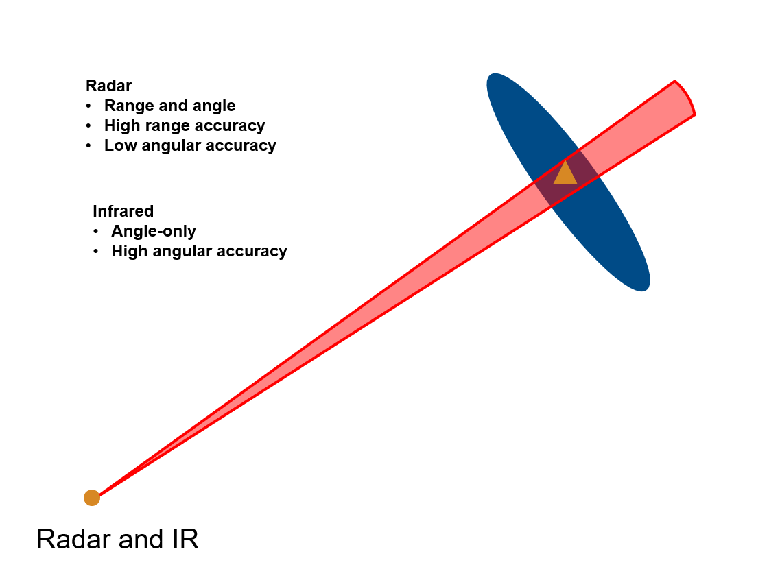
Radar and Infrared sensors provide complementary sensing capabilities to assist object tracking. Radar provides both range and angle measurements from an object and offers robust operation in all weather conditions. However, the angular accuracy of radar measurements is typically low. On the other hand, an infrared sensor provides only angular measurements from the object, but with a much higher angular accuracy as compared to a radar. Therefore, the fusion of radar and infrared measurements produces a more robust estimate about the location of an object. You can see visually, the fusion of angular covariance from infrared (red) and radar position covariance (blue) produces an intersection with a much smaller covariance as compared to the radar position covariance.

Setup Scenario and Visualization

In this section, you setup a marine scenario using the trackingScenario object. The scenario consists of small civilian boats close to the base station as well as a large cargo vessel exiting the harbor. You simulated these objects as point targets to generate at most one detection per object at every time step. You set the IsEarthCentered property of trackingScenario to true to simulate geo-referenced scenarios. Further, you use the geoTrajectory System object™ to specify trajectories of each object. You mount a mechanically scanning radar and infrared sensor on a stationary base station near the harbor. Thees sensors provide 180-degree coverage facing the east direction. For more details on the setup, see the helper function, helperCreateMarineGeoScenario, included with this example.

% Set random seed for reproducible results
rng(2022);

% Create scenario
scenario = helperCreateMarineGeoScenario;

You use the trackingGlobeViewer object to visualize the ground truth, instantaneous sensor coverages, detections, and the tracks generated by the tracker. To generate a birds-eye view of the scene, you set the camera position 7 kilometers above the ground using the campos object function. The image below shows the trajectory of all objects in the scene in blue and each blue diamond represents the starting position of the corresponding trajectory.

% Create a uifigure
sz = get(groot,'ScreenSize');
fig = uifigure(Position = [0.1*sz(3) 0.1*sz(4) 0.8*sz(3) 0.8*sz(4)]);

% Create tracking globe viewer
viewer = trackingGlobeViewer(fig,NumCovarianceSigma=1);

% Clear helper with persistence
clear helperPlotAngleOnlyDetection;

% Set position of camera
meanLat = mean(cellfun(@(x)x.Position(1),scenario.Platforms));
meanLong = mean(cellfun(@(x)x.Position(2),scenario.Platforms));
campos(viewer, [meanLat meanLong 7e3]);

% Plot all platforms
plotPlatform(viewer, [scenario.Platforms{:}],...
    TrajectoryMode="Full",...
    LineWidth=2,...
    Marker="d",...
    Color=[0.0745 0.6235 1.0000]);

% Take snapshot
drawnow;
snapshot(viewer);

Setup Tracker and Performance Metric

In this section, you set up a Gaussian-mixture probability hypothesis density (GM-PHD) multi-object tracker to track the objects using radar and infrared measurements. You also set up the OSPA-on-OSPA (optimal subpattern assignment) or OSPA(2) metric to evaluate the results from the tracker based on the simulated ground truth.

GM-PHD Tracker

You configure the multi-object tracker using the trackerPHD System object™, which uses a probability hypothesis density (PHD) filter to estimate the object states. In this example, you represent the state of each object using a point target model and use the Gaussian mixture representation of PHD filter (GM-PHD). The trackerPHD object requires definition of sensor configurations using the trackingSensorConfiguration object. You can directly create trackingSensorConfiguration objects from all the sensors in the scenario using the following command in MATLAB.

sensorConfigs = trackingSensorConfiguration(scenario);

Additionally, you need to set the SensorTransformFcn and FilterInitializationFcn properties after constructing the configurations depending on the state-space of the tracks. In this example, you use a constant velocity model (constvel, cvmeas) to describe the object motion. Therefore, you set the SensorTransformFcn to @cvmeas to enable transformation from a constant-velocity state space ($\left[\mathit{x}{\mathit{v}}_{\mathit{x}}\mathit{y}{\mathit{v}}_{\mathit{y}}\mathit{z}{\mathit{v}}_{\mathit{z}}\right]$) to the sensor's detectability space.

sensorConfigs{1}.SensorTransformFcn = @cvmeas;
sensorConfigs{2}.SensorTransformFcn = @cvmeas;

You configure the radar to initialize birth components from weakly-associated detections. As the infrared sensor does not provide complete observations of the objects, you configure it to add no birth components in the environment. You define these behaviors for the tracker by using the FilterInitializationFcn property of the trackingSensorConfiguration. For more information about birth density and the GM-PHD tracker, refer to the Algorithms section of trackerPHD.

The two helper functions, initRadarPHD and initIRPHD, use the initcvgmphd function to initialize the constant-velocity GM-PHD filter. As the radar and infrared sensors provide measurements of different sizes, you pad the infrared measurements with a dummy value to produce same size measurements as required by the tracker. The measurement model and its Jacobian defined using helper functions, cvmeasPadded and cvmeasjacPadded, inform the tracker about these dummy measurements.

% Define a function to initialize the PHD from each sensor
sensorConfigs{1}.FilterInitializationFcn = @initRadarPHD;
sensorConfigs{2}.FilterInitializationFcn = @initIRPHD;

% Construct the PHD tracker
tracker = trackerPHD(SensorConfigurations=sensorConfigs,...% Sensor configurations
    HasSensorConfigurationsInput=true,...% Sensor configurations change with time
    MaxNumComponents=5000,...% Maximum number of PHD components
    MergingThreshold=200,...% Merging Threshold
    AssignmentThreshold=150 ...% Threshold for adding birth components
    );

OSPA(2) Metric

In this example, you use the OSPA(2) metric to measure the performance of the tracker. The OSPA(2) metric allows you to evaluate the tracking performance by calculating a metric over history of tracks as opposed to instantaneous estimates in the traditional OSPA metric. As a result, the OSPA(2) metric penalizes phenomenon such as track switching and fragmentation more consistently. You configure the OSPA(2) metric by using the trackOSPAMetric object and setting the Metric property to "OSPA(2)". You choose absolute error in position as the base distance between a track and truth at a time instant by setting the Distance property to "posabserr".

% Define OSPA metric object
ospaMetric = trackOSPAMetric(Metric="OSPA(2)",...
    Distance="posabserr",...
    CutoffDistance=10);

Run Scenario and Track Objects

In this section, you run the scenario in a loop, generate detections and configurations from the sensor models and feed these data to the multi-object GM-PHD tracker. You pad infrared detections with a dummy measurement using the padDetectionsWithDummy helper function. To qualitatively assess the performance of the tracker, you visualize the results on the globe. To quantitatively assess the performance, you also evaluate the OSPA(2) metric.

% Initialize OSPA metric values
numSamples = scenario.StopTime*scenario.UpdateRate + 1;
ospa = nan(numSamples,1);
counter  = 1;

while advance(scenario)
    % Current time
    time = scenario.SimulationTime;
    
    % Generate detections and updated sensor configurations
    [detections, configs] = detect(scenario);

    % Make infrared measurements of same size
    detections = padDetectionsWithDummy(detections);

    % Update tracker
    tracks = tracker(detections, configs, time);
    
    % Update globe viewer
    updateDisplay(viewer, scenario, detections, tracks);
    
    % Obtain ground truth. Last platform is the sensing platform
    poses = platformPoses(scenario);
    gTruth = poses(1:end-1);

    % Calculate OSPA metric
    ospa(counter) = ospaMetric(tracks, gTruth);
    counter = counter + 1;

    % Take snapshot of Platform 10 at 5.9 seconds 
    if abs((time - 5.9)) < 0.05
        snap = zoomOnPlatform(viewer, scenario.Platforms{10}, 25);
    end
end

Results

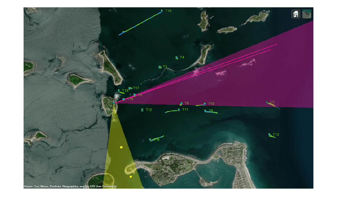
The image below shows the ground truth as well as the track history for all the platforms. The blue lines represent the ground truth trajectories and the green lines represent the tracks. The yellow and purple coverage areas represent the instantaneous coverage of the radar and infrared sensor, respectively. The purple lines represent the angle-only detections from the infrared sensor. Notice that the tracker is able to maintain tracks on all platforms.

snapshot(viewer);

In the next image you see the estimated track on the 8th platform in the scenario. Notice that the tracker maintains a track close to the actual position of the object and closely follows the true trajectory of the platform.

zoomOnPlatform(viewer, scenario.Platforms{8}, 250);

You can also quantitatively measure the tracking performance by plotting the OSPA(2) metric as a function of time. Notice that the OSPA(2) metric is less than 2 after 15 seconds of simulation. This indicates that the tracker is able to accurately track the positions of the objects. It also indicates that events like missed targets, false tracks as well as track switching and fragmentation did not occur during the simulation.

time = linspace(0,scenario.StopTime,numSamples);
plot(time, ospa,"LineWidth",2);
xlabel("Time(s)");
ylabel("Metric");

As mentioned, the accurate angle information from the infrared sensor allows the tracker to estimate the position of objects with much higher accuracy. The image below is the snapshot of a platform at about 5.9 seconds. From the image, you can observe the difference in the position uncertainty between the radar measurement and the track estimate. The track's uncertainty (denoted with a green ellipse) is much smaller as compared to the radar measurement uncertainty (denoted with a yellow ellipse). This demonstrates the effectiveness of fusing radar and infrared measurements.

imshow(snap);

Summary

In this example, you learned how to simulate a geo-referenced marine scenario and generate synthetic measurements using infrared and radar sensors. You also learned how to fuse position and angle-only measurements using a GM-PHD multi-object tracker. You assessed the tracking results by visualizing the tracks and ground truth on the globe and calculating the OSPA(2) metric.

Supporting Functions

initRadarPHD Initialize a constant velocity GM-PHD filter from radar detection.

function phd = initRadarPHD(varargin)
% initcvgmphd adds 1 component when detection is an input. It adds no
% components with no inputs. 
phd = initcvgmphd(varargin{:});
phd.ProcessNoise = 5*eye(3);

% Update measurement model to use padded measurements
phd.MeasurementFcn = @cvmeasPadded;
phd.MeasurementJacobianFcn = @cvmeasjacPadded;
end

initIRPHD Initialize a constant velocity GM-PHD filter from an IR detection.

function phd = initIRPHD(varargin)
% This adds no components
phd = initcvgmphd; 
phd.ProcessNoise = 5*eye(3);

% Update measurement model to use padded measurements
phd.MeasurementFcn = @cvmeasPadded; 
phd.MeasurementJacobianFcn = @cvmeasjacPadded;
end

cvmeasPadded Measurement model with padded dummy variable to output measurements as three-element vectors.

% Padded measurement model
function z = cvmeasPadded(x,varargin)
z = cvmeas(x,varargin{:});
numPads = 3 - size(z,1);
numStates = size(z,2);
z = [z;zeros(numPads,numStates)];
end

cvmeasjacPadded Jacobian of padded measurement model

% Jacobian of padded measurement model
function H = cvmeasjacPadded(x,varargin)
H = cvmeasjac(x,varargin{:});
numPads = 3 - size(H,1);
numStateElements = size(H,2);
H = [H;zeros(numPads,numStateElements)];
end

padDetectionsWithDummy Pads infrared detections with a dummy value.

function detections = padDetectionsWithDummy(detections)
for i = 1:numel(detections)
    % Infrared detections have SensorIndex = 2
    if detections{i}.SensorIndex == 2
        % Add dummy measurement
        detections{i}.Measurement = [detections{i}.Measurement;0];

        % A covariance value of 1/(2*pi) on the dummy measurement produces
        % the same Gaussian likelihood as the original measurement without
        % dummy
        detections{i}.MeasurementNoise = blkdiag(detections{i}.MeasurementNoise,1/(2*pi));
    end
end
end

updateDisplay Update the globe viewer

function updateDisplay(viewer, scenario, detections, tracks)

% Define position and velocity selectors
posSelector = [1 0 0 0 0 0;0 0 1 0 0 0;0 0 0 0 1 0];
velSelector = [0 1 0 0 0 0;0 0 0 1 0 0;0 0 0 0 0 1];

% Color order
colorOrder = [1.0000    1.0000    0.0667
    0.0745    0.6235    1.0000
    1.0000    0.4118    0.1608
    0.3922    0.8314    0.0745
    0.7176    0.2745    1.0000
    0.0588    1.0000    1.0000
    1.0000    0.0745    0.6510];

% Plot Platforms
plotPlatform(viewer, [scenario.Platforms{:}],'ECEF',Color=colorOrder(2,:),TrajectoryMode='Full');

% Plot Coverage
covConfig = coverageConfig(scenario);
covConfig(2).Range = 10e3;
plotCoverage(viewer,covConfig,'ECEF',Color=colorOrder([1 7],:),Alpha=0.2);

% Plot Detections
sIdx = cellfun(@(x)x.SensorIndex,detections);
plotDetection(viewer, detections(sIdx == 1), 'ECEF',Color=colorOrder(1,:));
helperPlotAngleOnlyDetection(viewer, detections(sIdx == 2),Color=colorOrder(7,:));

% Plot Tracks
plotTrack(viewer,tracks,'ECEF',PositionSelector=posSelector,...
    VelocitySelector=velSelector,LineWidth=2,Color=colorOrder(4,:));
drawnow;

end

zoomOnPlatform Take a snapshot of the platform from a certain height.

function varargout = zoomOnPlatform(viewer, platform, height)
currentPos = campos(viewer);
currentOrient = camorient(viewer);
pos = platform.Position;
campos(viewer,[pos(1) pos(2) height]);
drawnow;
[varargout{1:nargout}] = snapshot(viewer);
campos(viewer,currentPos);
camorient(viewer,currentOrient);
end