Define Trajectory Using Positions and Ground Speed

Overview

The waypointTrajectory object describes the motion of an object through a series of waypoints. The waypointTrajectory object is best used for describing an object that moves primarily in the horizontal x-y plane with a gradual climb or descent in the vertical direction. You can specify a waypointTrajectory object with and without the time-of-arrival information. With the time-of-arrival input, the object interpolates between the waypoints to generate a smooth trajectory. You can optionally specify the velocity at each waypoint in this case. Without the time-of-arrival input, you must specify the ground speed or velocity at each waypoint so that the object can determine the trajectory and times-of-arrival.

Specify Trajectory Lifetime (Start, Stop, and Wait)

You can specify the waypointTrajectory object to let it start and end at specific times. The trajectory reports valid trajectory states for any time within the time interval and reports not-a-number (NaN) values outside of that time interval. Utilizing this, you can define trajectories that last for only a small duration of time relative to other trajectories. You can also specify pause or wait time at specific waypoints. The trajectory remains at the same waypoint while in a wait state.

Based on whether the time-of-arrival information is available, you specify trajectory lifetime and pause durations in different ways.

Known Time-of-Arrival

When time-of-arrival information is known at each waypoint, you can specify it via the TimeOfArrival property.

In this case, the TimeOfArrival property defines the lifetime of the trajectory. As mentioned, the trajectory only reports valid values when you query the trajectory states, such as position and orientation, within the trajectory lifetime. Otherwise, the trajectory returns those values as NaNs.

To specify waiting at a specific position, repeat the position at two consecutive waypoints with different times of arrival. If you additionally specify velocities or ground speeds for these waypoints, the velocities or ground speeds must be zero.

In the following, you define a trajectory that starts at 2.6 seconds and ends at 28.3 seconds. The trajectory waits at location (41.1, 19.4, 0) from 11.5 seconds to 12.5 seconds. You achieve this by specifying the same coordinates for two consecutive waypoints at 11.5 second and 12.5 seconds.

waypoints1 = [49.6 -34.7  0
              47.1 -26.8  0
              41.5 -19.4  0
              41.5 -19.4  0
              28.7  -7.2  0
              20.2   1.0  0];
timeOfArrival1 = [2.6; 5.4; 11.5; 12.5; 24.3; 28.3];
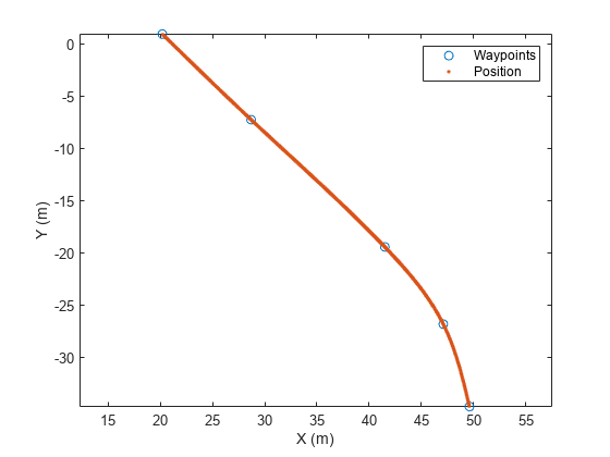
traj1 = waypointTrajectory(waypoints1,timeOfArrival1);

Next, plot the waypoints and trajectory from 0 to 30 seconds. The plot function ignores NaN values.

sampleTimes1 = linspace(0,30,1000);
[position1, orientation1, velocity1] = lookupPose(traj1,sampleTimes1);
plot(waypoints1(:,1),waypoints1(:,2),"o", ...
     position1(:,1), position1(:,2),".");
xlabel("X (m)");
ylabel("Y (m)");
axis equal
legend({"Waypoints","Position"})

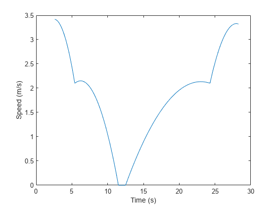
You can also plot the magnitude of the velocity (speed) as a function of time. From the results, the trajectory starts at 2.6 seconds and ends at 28 seconds. The trajectory position does not change from 11.5 to 12.5 seconds.

plot(sampleTimes1,vecnorm(velocity1,2,2));
xlabel("Time (s)");
ylabel("Speed (m/s)");

Unknown Time-of-Arrival

As of R2023a, the waypointTrajectory can automatically compute the time of arrival information if the velocity information is specified for each waypoint (by using the GroundSpeed property or the Velocity property). After the waypointTrajectory object is created, you can inspect the computed times-of-arrival stored in the TimeOfArrival property.

To let the trajectory start at a specific time, specify the start time in the InitialTime property. As a consequence, the trajectory also delays the trajectory stop time by the specified initial time. The trajectory reports NaN values outside the lifetime of the trajectory.

To let the trajectory wait at specific waypoints, specify nonzero values in the corresponding entries in the WaitTime property. Meanwhile, make sure that you specify the velocities at these points as zero.

In the following, you define a waypointTrajectory object using ground speed and specify the WaitTime property so that the trajectory waits at the third waypoint for one second.

waypoints2 = [49.6 -34.7  0
              47.1 -26.8  0
              41.5 -19.4  0
              28.7  -7.2  0
              20.2   1.0  0];
groundSpeed2 = [3; 3; 0; 3; 3];
waitTime2 = [0; 0; 1; 0; 0];
initialTime2 = timeOfArrival1(1);
traj2 = waypointTrajectory(waypoints2,GroundSpeed= groundSpeed2, ...
    WaitTime=waitTime2,InitialTime=initialTime2);

As previously, plot the waypoints and the positions. Note that the plot function ignores NaN values.

sampleTimes2 = linspace(0,30,1000);
[position2, orientation2, velocity2, acceleration2] = lookupPose(traj2, sampleTimes2);
plot(waypoints2(:,1),waypoints2(:,2),"o", ...
     position2(:,1), position2(:,2),".");
xlabel("X (m)");
ylabel("Y (m)");
axis equal
legend({"Waypoints","Position"})

Next, plot the speed as a function of time.

speed2 = vecnorm(velocity2,2,2);
plot(sampleTimes2, speed2);
xlabel("Time (s)");
ylabel("Speed (m/s)");

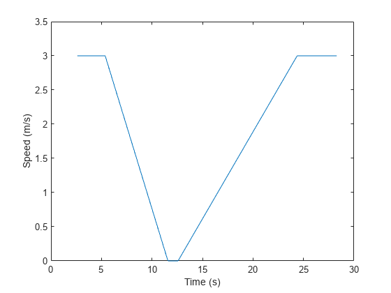
From the results, the trajectory starts at 2.6 seconds and ends at 28 seconds. The trajectory does not change from 11.5 to 12.5 seconds. Additionally, plot the acceleration in the forward direction of the motion as a function of time.

forward2 = rotatepoint(orientation2,repmat([1 0 0],size(velocity2,1),1));
forwardAcceleration2 = dot(acceleration2,forward2,2);
plot(sampleTimes2, forwardAcceleration2);
xlabel("Time (s)");
ylabel("Acceleration (m/s^2)");

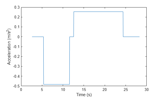
Observe that when using groundspeed (without time-of-arrival) the trajectory uses a piece-wise constant acceleration profile. The trajectory starts with no acceleration (constant speed) then decelerates after the second waypoint until it stops and pauses at 11.5 seconds. Then, it accelerates again at 12.5 seconds until the penultimate waypoint, where it resumes a constant speed.

Trajectory Smoothness

The waypointTrajectory has built-in interpolants that govern how quickly it traverses the path specified through the waypoints. The exact interpolants being used depends on whether the time-of-arrival information is available and other factors.

Known Time-of-Arrival

When time-of-arrival is known, the trajectory uses a shape preserving piecewise cubic spline to calculate the distance along the path of the curve as a function of time. If the groundspeed information is also known, the trajectory uses cubic Hermite interpolation, which allows a finer control of the speed of waypoints through which the path is traversed. You need to make sure that any groundspeed information provided to the waypointTrajectory object is consistent with the overall path and time of arrival information. Otherwise, the instantaneous groundspeeds used between waypoints may grossly overshoot or undershoot the desired speeds.

Unknown Time-of-Arrival

When the time of arrival information is unknown, the waypointTrajectory object uses piecewise constant acceleration between waypoints based on the specified groundspeed or velocity. As a result, the groundspeed reaches extrema at the waypoints, guaranteeing that the velocity will change in a monotonically increasing or decreasing fashion between waypoints.

The waypointTrajectory object also allows you to specify the limit of the jerk, which is the time derivative of the acceleration. In automotive applications, it is crucial to restrain the jerk limit over the course of the trajectory, because excessive jerks can result in an uncomfortable ride or even cause body injury for passengers. For example, passengers usually feel extremely uncomfortable when the jerk magnitude is beyond 0.9 m/s³.

If the JerkLimit property is specified, the trajectory produces a trapezoidal acceleration profile. Otherwise, it follows a piecewise-constant acceleration profile with a discontinuity in the acceleration value at the waypoints as shown in the last section.

Use the previous trajectory but set the jerk limit of the trajectory to 0.4 m/s³.

waypoints3 = waypoints2;
groundSpeed3 = groundSpeed2;
jerkLimit = 0.4;
waitTime3 = waitTime2;
initialTime3 = timeOfArrival1(1);
traj3 = waypointTrajectory(waypoints3,GroundSpeed=groundSpeed3,WaitTime=waitTime3, ...
    InitialTime=initialTime3,JerkLimit=jerkLimit);

To investigate the acceleration profile, plot the acceleration in the forward direction of motion.

sampleTimes3 = linspace(0,20,1000);
[position3, orientation3, velocity3, acceleration3] = lookupPose(traj3, sampleTimes3);
forward3 = rotatepoint(orientation3,repmat([1 0 0],size(velocity3,1),1));
forwardAcceleration3 = dot(acceleration3,forward3,2);
plot(sampleTimes3, forwardAcceleration3);
xlabel("Time (s)");
ylabel("Acceleration (m/s^2)");

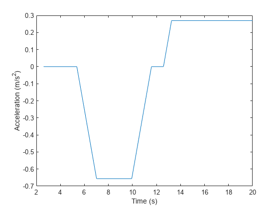
From the results, the trajectory produces a trapezoidal profile, which avoids instantaneous discontinuities in acceleration. Note that it is important to use realistic values for velocities of the waypoints. If the trajectory returns an error when you adjust the jerk limit, it is possible for the trajectory to return error because the jerk limit is not achievable given the velocity or groundspeed. In this case, you can try adding more waypoints or reducing the difference in speeds between the problematic waypoints.

Summary

In this example, you learned how to construct a waypointTrajectory object with and without time-of-arrival information. You also explored ways to control trajectory lifetime and its smoothness.