Main Content

waypointTrajectory

Waypoint trajectory generator

Description

The waypointTrajectory System object™ generates trajectories based on specified waypoints. When you create the System object, you can choose to specify the time of arrival, velocity, or ground speed at each waypoint. You can optionally specify other properties such as orientation at each waypoint. See Algorithms for more details.

To generate a trajectory from waypoints:

  1. Create the waypointTrajectory object and set its properties.

  2. Call the object as if it were a function.

To learn more about how System objects work, see What Are System Objects?.

Creation

Description

trajectory = waypointTrajectory returns a System object, trajectory, that generates a trajectory based on default stationary waypoints.

example

trajectory = waypointTrajectory(Waypoints,TimeOfArrival) specifies the time of arrival at which the generated trajectory passes through each waypoint. See the TimeOfArrival property for more details.

Tip

When you specify the TimeOfArrival argument, you must not specify these properties:

  • JerkLimit

  • InitialTime

  • WaitTime

example

trajectory = waypointTrajectory(Waypoints,GroundSpeed=groundSpeed) specifies the ground speed at which the generated trajectory passes through at each waypoint. See the GroundSpeed property for more details.

example

trajectory = waypointTrajectory(Waypoints,Velocities=velocities) specifies the velocity at which the generated trajectory passes through at each waypoint. See the Velocities property for more details.

trajectory = waypointTrajectory(___,Name=Value) sets each property by using name-value arguments. Unspecified properties have default or inferred values. You can use this syntax with any of the previous syntaxes.

example

Example: trajectory = waypointTrajectory([10,10,0;20,20,0;20,20,10],[0,0.5,10]) creates a waypoint trajectory System object, trajectory, that starts at waypoint [10,10,0], and then passes through [20,20,0] after 0.5 seconds and [20,20,10] after 10 seconds.

Properties

expand all

Unless otherwise indicated, properties are nontunable, which means you cannot change their values after calling the object. Objects lock when you call them, and the release function unlocks them.

If a property is tunable, you can change its value at any time.

For more information on changing property values, see System Design in MATLAB Using System Objects.

Sample rate of trajectory in Hz, specified as a positive scalar.

Tunable: Yes

Data Types: double

Number of samples per output frame, specified as a positive scalar integer.

Data Types: double

This property is read-only.

Positions in the navigation coordinate system in meters, specified as an N-by-3 matrix. The columns of the matrix correspond to the first, second, and third axes, respectively. The rows of the matrix, N, correspond to individual waypoints.

Tip

To let the trajectory wait at a specific waypoint, use one of the two options:

  • If you specified the TimeOfArrival input argument, repeat the waypoint coordinate in two consecutive rows.

  • If you did not specify the TimeOfArrival input argument, specify the wait time using the WaitTime property.

You can only set this property as a name-value argument during construction.

Data Types: double

This property is read-only.

Time corresponding to arrival at each waypoint in seconds, specified as an N-element column vector. The number of samples, N, must be the same as the number of samples (rows) defined by Waypoints.

You can only set this property as a name-value argument during construction.

Dependencies

To set this property, you must not specify these properties:

  • JerkLimit

  • InitialTime

  • WaitTime

Data Types: double

This property is read-only.

Velocity in the navigation coordinate system at each waypoint in meters per second, specified as an N-by-3 matrix. The columns of the matrix correspond to the first, second, and third axes, respectively. The number of samples, N, must be the same as the number of samples (rows) defined by Waypoints.

If the velocity is specified as a non-zero value, the object automatically calculates the course of the trajectory based on the velocity. If the velocity is specified as zero, the object infers the course of the trajectory from adjacent waypoints.

You can only set this property as a name-value argument during construction.

Data Types: double

This property is read-only.

Horizontal direction of travel, specified as an N-element real vector in degrees. The number of samples, N, must be the same as the number of samples (rows) defined by Waypoints. If neither Velocities nor Course is specified, course is inferred from the waypoints.

You can only set this property as a name-value argument during construction.

Dependencies

To set this property, the Velocities property must not be specified.

Data Types: double

This property is read-only.

Groundspeed at each waypoint, specified as an N-element real vector in m/s. If the property is not specified, it is inferred from the waypoints. The number of samples, N, must be the same as the number of samples (rows) defined by Waypoints.

  • To render forward motion, specify positive ground speed values.

  • To render backward motion, specify negative ground speed values.

  • To render reverse motion, separate positive and negative groundspeed values by a zero groundspeed value.

You can only set this property as a name-value argument during construction.

Dependencies

To set this property, the Velocities property must not be specified.

Data Types: double

This property is read-only.

Climb Rate at each waypoint in meters per second, specified as an N-element real vector. The number of samples, N, must be the same as the number of samples (rows) defined by Waypoints. If neither Velocities nor Course is specified, climb rate is inferred from the waypoints.

You can only set this property as a name-value argument during construction.

Dependencies

To set this property, the Velocities property must not be specified.

Data Types: double

This property is read-only.

Longitudinal jerk limit, specified as a positive scalar in m/s3. Jerk is the time derivative of the acceleration. When you specify this property, the object produces a horizontal trapezoidal acceleration profile based on the jerk limit. If the waypointTrajectory object cannot achieve the specified JerkLimit, the object issues an error.

You can only set this property as a name-value argument during construction.

Dependencies

To set this property, the TimeOfArrival property must not be specified.

Data Types: double

This property is read-only.

Time before the trajectory starts, specified as a nonnegative scalar in seconds. The object reports quantities, such as position and velocity, as NaN before the trajectory starts.

You can only set this property as a name-value argument during construction.

Dependencies

To set this property, the TimeOfArrival property must not be specified. Instead, you must specify either the GroundSpeed or Velocities property when creating the object.

Data Types: double

This property is read-only.

Wait time at each waypoint, specified as an N-element vector of nonnegative scalars. N must be the same as the number of samples (rows) defined by Waypoints.

You can only set this property as a name-value argument during construction.

Dependencies

To set this property, the TimeOfArrival property must not be specified.

If you specified the TimeOfArrival property, then you cannot specify wait time through this property. Instead, specify wait time by repeating the waypoint coordinate in two consecutive rows in the Waypoints property.

Data Types: double

This property is read-only.

Orientation at each waypoint, specified as an N-element quaternion column vector or 3-by-3-by-N array of real numbers. Each quaternion must have a norm of 1. Each 3-by-3 rotation matrix must be an orthonormal matrix. The number of quaternions or rotation matrices, N, must be the same as the number of samples (rows) defined by Waypoints.

If Orientation is specified by quaternions, the underlying class must be double.

You can only set this property as a name-value argument during construction.

Data Types: double

This property is read-only.

Align pitch angle with the direction of motion, specified as true or false. When specified as true, the pitch angle automatically aligns with the direction of motion. If specified as false, the pitch angle is set to zero (level orientation).

You can only set this property as a name-value argument during construction.

Dependencies

To set this property, the Orientation property must not be specified.

This property is read-only.

Align roll angle to counteract the centripetal force, specified as true or false. When specified as true, the roll angle automatically counteracts the centripetal force. If specified as false, the roll angle is set to zero (flat orientation).

You can only set this property as a name-value argument during construction.

Dependencies

To set this property, the Orientation property must not be specified.

This property is read-only.

Reference frame of the trajectory, specified as 'NED' (North-East-Down) or 'ENU' (East-North-Up).

You can only set this property as a name-value argument during construction.

Usage

Description

[position,orientation,velocity,acceleration,angularVelocity] = trajectory() outputs a frame of trajectory data based on specified creation arguments and properties.

example

Output Arguments

expand all

Position in the local navigation coordinate system in meters, returned as an M-by-3 matrix.

M is specified by the SamplesPerFrame property.

Data Types: double

Orientation in the local navigation coordinate system, returned as an M-by-1 quaternion column vector or a 3-by-3-by-M real array.

Each quaternion or 3-by-3 rotation matrix is a frame rotation from the local navigation coordinate system to the current body coordinate system.

M is specified by the SamplesPerFrame property.

Data Types: double

Velocity in the local navigation coordinate system in meters per second, returned as an M-by-3 matrix.

M is specified by the SamplesPerFrame property.

Data Types: double

Acceleration in the local navigation coordinate system in meters per second squared, returned as an M-by-3 matrix.

M is specified by the SamplesPerFrame property.

Data Types: double

Angular velocity in the local navigation coordinate system in radians per second, returned as an M-by-3 matrix.

M is specified by the SamplesPerFrame property.

Data Types: double

Object Functions

To use an object function, specify the System object as the first input argument. For example, to release system resources of a System object named obj, use this syntax:

release(obj)

expand all

waypointInfoGet waypoint information table
lookupPoseObtain pose information for certain time
perturbationsPerturbation defined on object
perturbApply perturbations to object
cloneCreate duplicate System object
stepRun System object algorithm
releaseRelease resources and allow changes to System object property values and input characteristics
resetReset internal states of System object
isDoneEnd-of-data status

Examples

collapse all

trajectory = waypointTrajectory
trajectory = 
  waypointTrajectory with properties:

         SampleRate: 100
    SamplesPerFrame: 1
          Waypoints: [2x3 double]
      TimeOfArrival: [2x1 double]
         Velocities: [2x3 double]
             Course: [2x1 double]
        GroundSpeed: [2x1 double]
          ClimbRate: [2x1 double]
        Orientation: [2x1 quaternion]
          AutoPitch: 0
           AutoBank: 0
     ReferenceFrame: 'NED'

Inspect the default waypoints and times of arrival by calling waypointInfo. By default, the waypoints indicate a stationary position for one second.

waypointInfo(trajectory)
ans=2×2 table
    TimeOfArrival     Waypoints 
    _____________    ___________

          0          0    0    0
          1          0    0    0

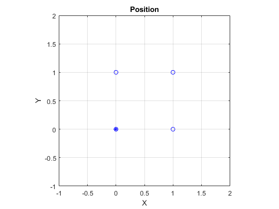
Create a square trajectory and examine the relationship between waypoint constraints, sample rate, and the generated trajectory.

Create a square trajectory by defining the vertices of the square. Define the orientation at each waypoint as pointing in the direction of motion. Specify a 1 Hz sample rate and use the default SamplesPerFrame of 1.

waypoints = [0,0,0; ... % Initial position
             0,1,0; ...
             1,1,0; ...
             1,0,0; ...
             0,0,0];    % Final position

toa = 0:4; % time of arrival

orientation = quaternion([0,0,0; ...
                          45,0,0; ...
                          135,0,0; ...
                          225,0,0; ...
                          0,0,0], ...
                          "eulerd","ZYX","frame");

trajectory = waypointTrajectory(waypoints, ...
    TimeOfArrival=toa, ...
    Orientation=orientation, ...
    SampleRate=1);

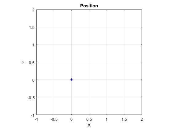
Create a figure and plot the initial position of the platform.

figure(1)
plot(waypoints(1,1),waypoints(1,2),"b*")
title("Position")
axis([-1,2,-1,2])
axis square
xlabel("X")
ylabel("Y")
grid on
hold on

In a loop, step through the trajectory to output the current position and current orientation. Plot the current position and log the orientation. Use pause to mimic real-time processing.

orientationLog = zeros(toa(end)*trajectory.SampleRate,1,"quaternion");
count = 1;
while ~isDone(trajectory)
   [currentPosition,orientationLog(count)] = trajectory();

   plot(currentPosition(1),currentPosition(2),"bo")

   pause(trajectory.SamplesPerFrame/trajectory.SampleRate)
   count = count + 1;
end
hold off

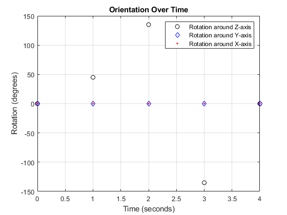
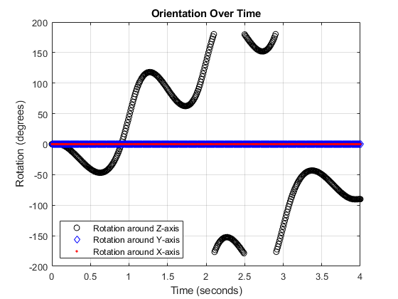
Convert the orientation quaternions to Euler angles for easy interpretation, and then plot orientation over time.

figure(2)
eulerAngles = eulerd([orientation(1);orientationLog],"ZYX","frame");
plot(toa,eulerAngles(:,1),"ko", ...
     toa,eulerAngles(:,2),"bd", ...
     toa,eulerAngles(:,3),"r.");
title("Orientation Over Time")
legend("Rotation around Z-axis","Rotation around Y-axis","Rotation around X-axis")
xlabel("Time (seconds)")
ylabel("Rotation (degrees)")
grid on

So far, the trajectory object has only output the waypoints that were specified during construction. To interpolate between waypoints, increase the sample rate to a rate faster than the time of arrivals of the waypoints. Set the trajectory sample rate to 100 Hz and call reset.

trajectory.SampleRate = 100;
reset(trajectory)

Create a figure and plot the initial position of the platform. In a loop, step through the trajectory to output the current position and current orientation. Plot the current position and log the orientation. Use pause to mimic real-time processing.

figure(1)
plot(waypoints(1,1),waypoints(1,2),"b*")
title("Position")
axis([-1,2,-1,2])
axis square
xlabel("X")
ylabel("Y")
grid on
hold on

orientationLog = zeros(toa(end)*trajectory.SampleRate,1,"quaternion");
count = 1;
while ~isDone(trajectory)
   [currentPosition,orientationLog(count)] = trajectory();

   plot(currentPosition(1),currentPosition(2),"bo")

   pause(trajectory.SamplesPerFrame/trajectory.SampleRate)
   count = count + 1;
end
hold off

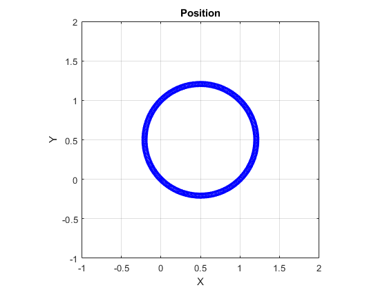
The trajectory output now appears circular. This is because the waypointTrajectory System object™ minimizes the acceleration and angular velocity when interpolating, which results in smoother, more realistic motions in most scenarios.

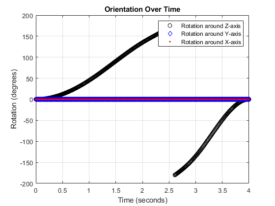
Convert the orientation quaternions to Euler angles for easy interpretation, and then plot orientation over time. The orientation is also interpolated.

figure(2)
eulerAngles = eulerd([orientation(1);orientationLog],"ZYX","frame");
t = 0:1/trajectory.SampleRate:4;
plot(t,eulerAngles(:,1),"ko", ...
     t,eulerAngles(:,2),"bd", ...
     t,eulerAngles(:,3),"r.");
title("Orientation Over Time")
legend("Rotation around Z-axis","Rotation around Y-axis","Rotation around X-axis")
xlabel("Time (seconds)")
ylabel("Rotation (degrees)")
grid on

The waypointTrajectory algorithm interpolates the waypoints to create a smooth trajectory. To return to the square trajectory, provide more waypoints, especially around sharp changes. To track corresponding times, waypoints, and orientation, specify all the trajectory info in a single matrix.

               % Time, Waypoint, Orientation
trajectoryInfo = [0,   0,0,0,    0,0,0; ... % Initial position
                  0.1, 0,0.1,0,  0,0,0; ...

                  0.9, 0,0.9,0,  0,0,0; ...
                  1,   0,1,0,    45,0,0; ...
                  1.1, 0.1,1,0,  90,0,0; ...

                  1.9, 0.9,1,0,  90,0,0; ...
                  2,   1,1,0,    135,0,0; ...
                  2.1, 1,0.9,0,  180,0,0; ...

                  2.9, 1,0.1,0,  180,0,0; ...
                  3,   1,0,0,    225,0,0; ...
                  3.1, 0.9,0,0,  270,0,0; ...

                  3.9, 0.1,0,0,  270,0,0; ...
                  4,   0,0,0,    270,0,0];    % Final position

trajectory = waypointTrajectory(trajectoryInfo(:,2:4), ...
    TimeOfArrival=trajectoryInfo(:,1), ...
    Orientation=quaternion(trajectoryInfo(:,5:end),"eulerd","ZYX","frame"), ...
    SampleRate=100);

Create a figure and plot the initial position of the platform. In a loop, step through the trajectory to output the current position and current orientation. Plot the current position and log the orientation. Use pause to mimic real-time processing.

figure(1)
plot(waypoints(1,1),waypoints(1,2),"b*")
title("Position")
axis([-1,2,-1,2])
axis square
xlabel("X")
ylabel("Y")
grid on
hold on

orientationLog = zeros(toa(end)*trajectory.SampleRate,1,"quaternion");
count = 1;
while ~isDone(trajectory)
   [currentPosition,orientationLog(count)] = trajectory();

   plot(currentPosition(1),currentPosition(2),"bo")

   pause(trajectory.SamplesPerFrame/trajectory.SampleRate)
   count = count+1;
end
hold off

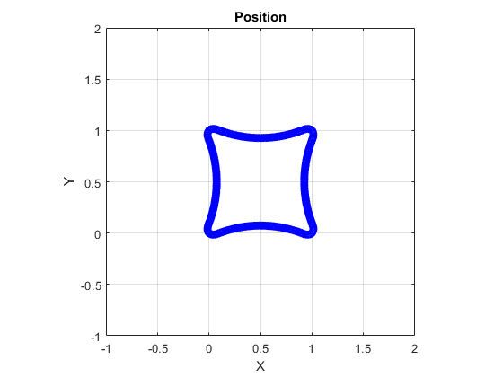
The trajectory output now appears more square-like, especially around the vertices with waypoints.

Convert the orientation quaternions to Euler angles for easy interpretation, and then plot orientation over time.

figure(2)
eulerAngles = eulerd([orientation(1);orientationLog],"ZYX","frame");
t = 0:1/trajectory.SampleRate:4;
eulerAngles = plot(t,eulerAngles(:,1),"ko", ...
                   t,eulerAngles(:,2),"bd", ...
                   t,eulerAngles(:,3),"r.");
title("Orientation Over Time")
legend("Rotation around Z-axis", ...
       "Rotation around Y-axis", ...
       "Rotation around X-axis", ...
       "Location", "SouthWest")
xlabel("Time (seconds)")
ylabel("Rotation (degrees)")
grid on

This example shows how to create an arc trajectory using the waypointTrajectory System object™. waypointTrajectory creates a path through specified waypoints that minimizes acceleration and angular velocity. After creating an arc trajectory, you restrict the trajectory to be within preset bounds.

Create an Arc Trajectory

Define a constraints matrix consisting of waypoints, times of arrival, and orientation for an arc trajectory. The generated trajectory passes through the waypoints at the specified times with the specified orientation. The waypointTrajectory System object requires orientation to be specified using quaternions or rotation matrices. Convert the Euler angles saved in the constraints matrix to quaternions when specifying the Orientation property.

          % Arrival, Waypoints, Orientation
constraints = [0,    20,20,0,    90,0,0;
               3,    50,20,0,    90,0,0;
               4,    58,15.5,0,  162,0,0;
               5.5,  59.5,0,0    180,0,0];

trajectory = waypointTrajectory(constraints(:,2:4), ...
    TimeOfArrival=constraints(:,1), ...
    Orientation=quaternion(constraints(:,5:7),"eulerd","ZYX","frame"));

Call waypointInfo on trajectory to return a table of your specified constraints. The creation properties Waypoints, TimeOfArrival, and Orientation are variables of the table. The table is convenient for indexing while plotting.

tInfo = waypointInfo(trajectory)
tInfo =

  4x3 table

    TimeOfArrival         Waypoints            Orientation   
    _____________    ____________________    ________________

           0           20      20       0    {1x1 quaternion}
           3           50      20       0    {1x1 quaternion}
           4           58    15.5       0    {1x1 quaternion}
         5.5         59.5       0       0    {1x1 quaternion}

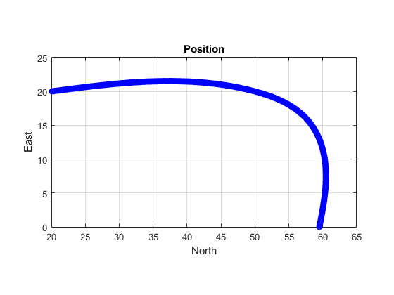
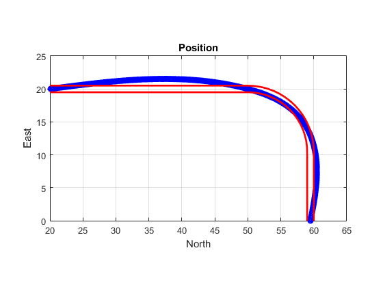
The trajectory object outputs the current position, velocity, acceleration, and angular velocity at each call. Call trajectory in a loop and plot the position over time. Cache the other outputs.

figure(1)
plot(tInfo.Waypoints(1,1),tInfo.Waypoints(1,2),"b*")
title("Position")
axis([20,65,0,25])
xlabel("North")
ylabel("East")
grid on
daspect([1 1 1])
hold on

orient = zeros(tInfo.TimeOfArrival(end)*trajectory.SampleRate,1,"quaternion");
vel = zeros(tInfo.TimeOfArrival(end)*trajectory.SampleRate,3);
acc = vel;
angVel = vel;

count = 1;
while ~isDone(trajectory)
   [pos,orient(count),vel(count,:),acc(count,:),angVel(count,:)] = trajectory();

   plot(pos(1),pos(2),"bo")

   pause(trajectory.SamplesPerFrame/trajectory.SampleRate)
   count = count + 1;
end

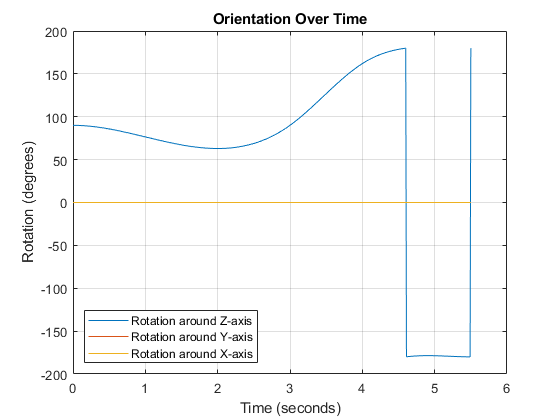
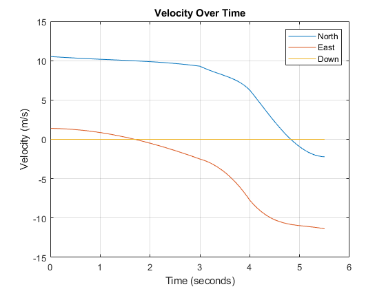
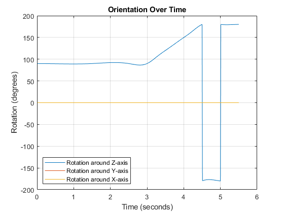
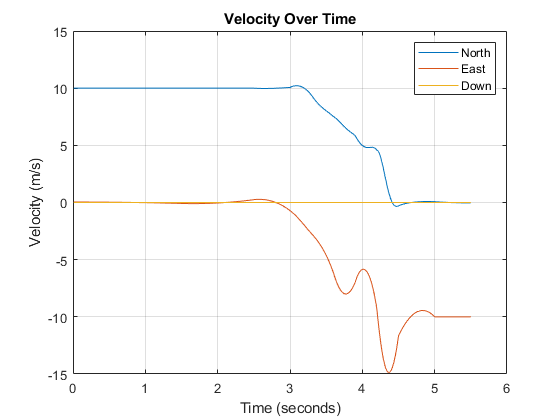
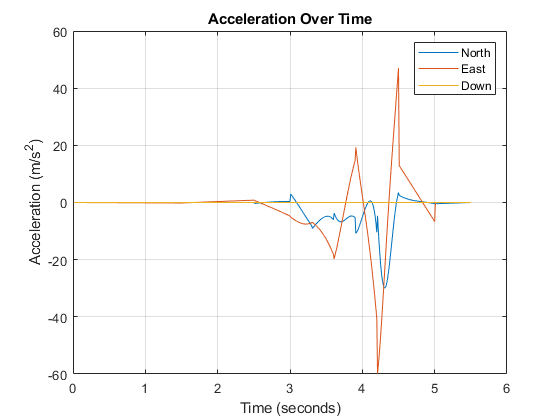
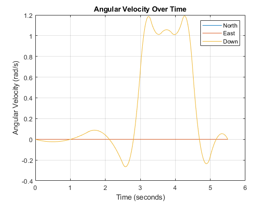
Inspect the orientation, velocity, acceleration, and angular velocity over time. The waypointTrajectory System object™ creates a path through the specified constraints that minimized acceleration and angular velocity.

figure(2)
timeVector = 0:(1/trajectory.SampleRate):tInfo.TimeOfArrival(end);
eulerAngles = eulerd([tInfo.Orientation{1};orient],"ZYX","frame");
plot(timeVector,eulerAngles(:,1), ...
     timeVector,eulerAngles(:,2), ...
     timeVector,eulerAngles(:,3));
title("Orientation Over Time")
legend("Rotation around Z-axis", ...
       "Rotation around Y-axis", ...
       "Rotation around X-axis", ...
       "Location","southwest")
xlabel("Time (seconds)")
ylabel("Rotation (degrees)")
grid on

figure(3)
plot(timeVector(2:end),vel(:,1), ...
     timeVector(2:end),vel(:,2), ...
     timeVector(2:end),vel(:,3));
title("Velocity Over Time")
legend("North","East","Down")
xlabel("Time (seconds)")
ylabel("Velocity (m/s)")
grid on

figure(4)
plot(timeVector(2:end),acc(:,1), ...
     timeVector(2:end),acc(:,2), ...
     timeVector(2:end),acc(:,3));
title("Acceleration Over Time")
legend("North","East","Down","Location","southwest")
xlabel("Time (seconds)")
ylabel("Acceleration (m/s^2)")
grid on

figure(5)
plot(timeVector(2:end),angVel(:,1), ...
     timeVector(2:end),angVel(:,2), ...
     timeVector(2:end),angVel(:,3));
title("Angular Velocity Over Time")
legend("North","East","Down")
xlabel("Time (seconds)")
ylabel("Angular Velocity (rad/s)")
grid on

Restrict Arc Trajectory Within Preset Bounds

You can specify additional waypoints to create trajectories within given bounds. Create upper and lower bounds for the arc trajectory.

figure(1)
xUpperBound = [(20:50)';50+10*sin(0:0.1:pi/2)';60*ones(11,1)];
yUpperBound = [20.5.*ones(31,1);10.5+10*cos(0:0.1:pi/2)';(10:-1:0)'];

xLowerBound = [(20:49)';50+9*sin(0:0.1:pi/2)';59*ones(11,1)];
yLowerBound = [19.5.*ones(30,1);10.5+9*cos(0:0.1:pi/2)';(10:-1:0)'];

plot(xUpperBound,yUpperBound,"r","LineWidth",2);
plot(xLowerBound,yLowerBound,"r","LineWidth",2)

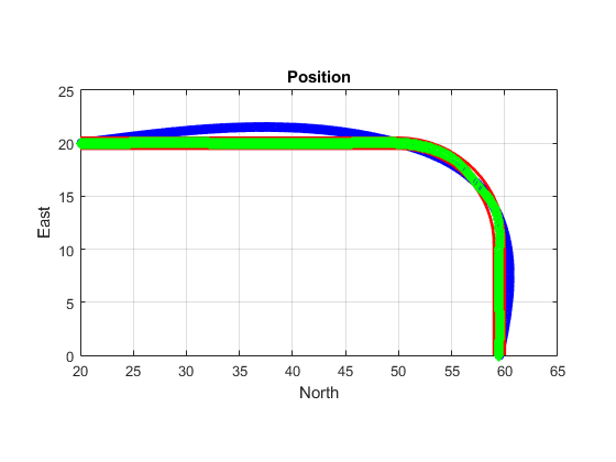
To create a trajectory within the bounds, add additional waypoints. Create a new waypointTrajectory System object™, and then call it in a loop to plot the generated trajectory. Cache the orientation, velocity, acceleration, and angular velocity output from the trajectory object.

            % Time,  Waypoint,     Orientation
constraints = [0,    20,20,0,      90,0,0;
               1.5,  35,20,0,      90,0,0;
               2.5   45,20,0,      90,0,0;
               3,    50,20,0,      90,0,0;
               3.3,  53,19.5,0,    108,0,0;
               3.6,  55.5,18.25,0, 126,0,0;
               3.9,  57.5,16,0,    144,0,0;
               4.2,  59,14,0,      162,0,0;
               4.5,  59.5,10,0     180,0,0;
               5,    59.5,5,0      180,0,0;
               5.5,  59.5,0,0      180,0,0];

trajectory = waypointTrajectory(constraints(:,2:4), ...
    TimeOfArrival=constraints(:,1), ...
    Orientation=quaternion(constraints(:,5:7),"eulerd","ZYX","frame"));
tInfo = waypointInfo(trajectory);

figure(1)
plot(tInfo.Waypoints(1,1),tInfo.Waypoints(1,2),"b*")

count = 1;
while ~isDone(trajectory)
   [pos,orient(count),vel(count,:),acc(count,:),angVel(count,:)] = trajectory();

   plot(pos(1),pos(2),"gd")

   pause(trajectory.SamplesPerFrame/trajectory.SampleRate)
   count = count + 1;
end

The generated trajectory now fits within the specified boundaries. Visualize the orientation, velocity, acceleration, and angular velocity of the generated trajectory.

figure(2)
timeVector = 0:(1/trajectory.SampleRate):tInfo.TimeOfArrival(end);
eulerAngles = eulerd(orient,"ZYX","frame");
plot(timeVector(2:end),eulerAngles(:,1), ...
     timeVector(2:end),eulerAngles(:,2), ...
     timeVector(2:end),eulerAngles(:,3));
title("Orientation Over Time")
legend("Rotation around Z-axis", ...
       "Rotation around Y-axis", ...
       "Rotation around X-axis", ...
       "Location","southwest")
xlabel("Time (seconds)")
ylabel("Rotation (degrees)")
grid on

figure(3)
plot(timeVector(2:end),vel(:,1), ...
     timeVector(2:end),vel(:,2), ...
     timeVector(2:end),vel(:,3));
title("Velocity Over Time")
legend("North","East","Down")
xlabel("Time (seconds)")
ylabel("Velocity (m/s)")
grid on

figure(4)
plot(timeVector(2:end),acc(:,1), ...
     timeVector(2:end),acc(:,2), ...
     timeVector(2:end),acc(:,3));
title("Acceleration Over Time")
legend("North","East","Down")
xlabel("Time (seconds)")
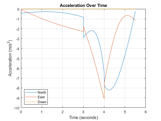
ylabel("Acceleration (m/s^2)")
grid on

figure(5)
plot(timeVector(2:end),angVel(:,1), ...
     timeVector(2:end),angVel(:,2), ...
     timeVector(2:end),angVel(:,3));
title("Angular Velocity Over Time")
legend("North","East","Down")
xlabel("Time (seconds)")
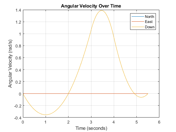
ylabel("Angular Velocity (rad/s)")
grid on

Note that while the generated trajectory now fits within the spatial boundaries, the acceleration and angular velocity of the trajectory are somewhat erratic. This is due to over-specifying waypoints.

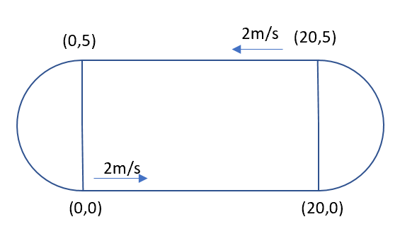
Consider a racetrack trajectory as the following.

The four corner points of the trajectory are (0,0,0), (20,0,0), (20,5,0) and (0,5,0) in meters, respectively. Therefore, specify the waypoints of a loop as:

wps = [0 0 0;
      20 0 0;
      20 5 0;
      0  5 0;
      0  0 0];

Assume the trajectory has a constant speed of 2 m/s, and thus the velocities at the five waypoints are:

vels = [2 0 0;
        2 0 0;
       -2 0 0;
       -2 0 0;
        2 0 0];

The time of arrival for the five waypoints is:

t = cumsum([0 20/2 5*pi/2/2 20/2 5*pi/2/2]');

The orientation of the trajectory at the five waypoints are:

eulerAngs = [0 0 0;
             0 0 0;
           180 0 0;
           180 0 0;
             0 0 0]; % Angles in degrees.
% Convert Euler angles to quaternions.
quats = quaternion(eulerAngs,"eulerd","ZYX","frame");

Specify the sample rate as 100 for smoothing trajectory lines.

fs = 100;

Construct the waypointTrajectory.

traj = waypointTrajectory(wps,SampleRate=fs, ...
        Velocities=vels,...
        TimeOfArrival=t,...
        Orientation=quats);

Sample and plot the trajectory.

[pos, orient, vel, acc, angvel] = traj();
i = 1;

spf = traj.SamplesPerFrame;
while ~isDone(traj)
    idx = (i+1):(i+spf);
    [pos(idx,:), orient(idx,:), ...
        vel(idx,:), acc(idx,:), angvel(idx,:)] = traj();
    i = i+spf;
end

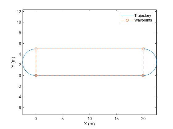
Plot the trajectory and the specified waypoints.

plot(pos(:,1),pos(:,2), wps(:,1),wps(:,2), "--o")
xlabel("X (m)")
ylabel("Y (m)")
zlabel("Z (m)")
legend({"Trajectory", "Waypoints"})
axis equal

Figure contains an axes object. The axes object with xlabel X (m), ylabel Y (m) contains 2 objects of type line. These objects represent Trajectory, Waypoints.

Create a waypointTrajectory object that connects two waypoints. The velocity of the trajectory at the two waypoints is 0 m/s and 10 m/s, respectively. Restrict the jerk limit to 0.5 m/s3 to enable the trapezoidal acceleration profile.

waypoints = [0  0  0;
            10 50 10];
speeds = [0 10];
jerkLimit = 0.5;
trajectory = waypointTrajectory(waypoints,GroundSpeed=speeds,JerkLimit=jerkLimit);

Obtain the initial time and final time of the trajectory by querying the TimeOfArrival property. Create time stamps to sample the trajectory.

t0 = trajectory.TimeOfArrival(1);
tf = trajectory.TimeOfArrival(end);
sampleTimes = linspace(t0,tf,100);

Obtain the position, velocity, and acceleration information at these sampled time stamps using the lookupPose object function.

[position,~,velocity,acceleration,~] = lookupPose(trajectory,sampleTimes);

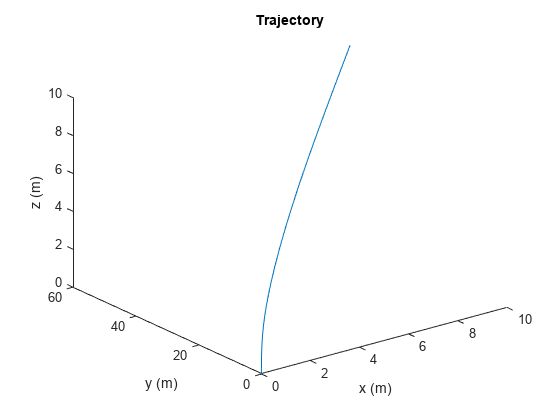
Plot the trajectory.

figure()
plot3(position(:,1),position(:,2),position(:,3))
xlabel("x (m)")
ylabel("y (m)")
zlabel("z (m)")
title("Trajectory")

Figure contains an axes object. The axes object with title Trajectory, xlabel x (m), ylabel y (m) contains an object of type line.

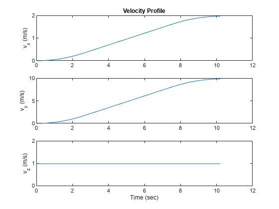
Plot the velocity profile.

figure()
subplot(3,1,1)
plot(sampleTimes,velocity(:,1));
ylabel("v_x (m/s)")
title("Velocity Profile")
subplot(3,1,2)
plot(sampleTimes,velocity(:,2));
ylabel("v_y (m/s)")
subplot(3,1,3)
plot(sampleTimes,velocity(:,3));
ylabel("v_z (m/s)")
xlabel("Time (sec)")

Figure contains 3 axes objects. Axes object 1 with title Velocity Profile, ylabel v_x (m/s) contains an object of type line. Axes object 2 with ylabel v_y (m/s) contains an object of type line. Axes object 3 with xlabel Time (sec), ylabel v_z (m/s) contains an object of type line.

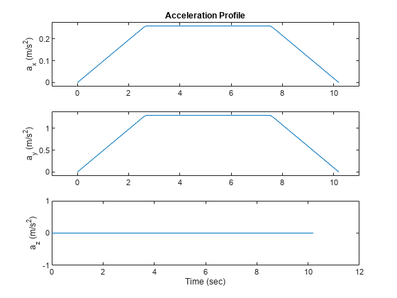
Plot the acceleration profile. From the results, the acceleration profile of the planar motion is trapezoidal.

figure()
subplot(3,1,1)
plot(sampleTimes,acceleration(:,1));
axis padded
ylabel("a_x (m/s^2)")
title("Acceleration Profile")
subplot(3,1,2)
plot(sampleTimes,acceleration(:,2));
ylabel("a_y (m/s^2)")
axis padded
subplot(3,1,3)
plot(sampleTimes,acceleration(:,3));
ylabel("a_z (m/s^2)")
xlabel("Time (sec)")

Figure contains 3 axes objects. Axes object 1 with title Acceleration Profile, ylabel a_x (m/s^2) contains an object of type line. Axes object 2 with ylabel a_y (m/s^2) contains an object of type line. Axes object 3 with xlabel Time (sec), ylabel a_z (m/s^2) contains an object of type line.

Algorithms

The waypointTrajectory System object defines a trajectory that smoothly passes through waypoints. The trajectory connects the waypoints through an interpolation that assumes the gravity direction expressed in the trajectory reference frame is constant. Generally, you can use waypointTrajectory to model platform or vehicle trajectories within a hundreds of kilometers distance span.

The planar path of the trajectory (the x-y plane projection) consists of piecewise, clothoid curves. The curvature of the curve between two consecutive waypoints varies linearly with the curve length between them. The tangent direction of the path at each waypoint is chosen to minimize discontinuities in the curvature, unless the course is specified explicitly via the Course property or implicitly via the Velocities property. Once the path is established, the object uses cubic Hermite interpolation to compute the location of the vehicle throughout the path as a function of time and the planar distance traveled. If the JerkLimit property is specified, the objects produces a horizontal trapezoidal acceleration profile for any segment that is between two waypoints. The trapezoidal acceleration profile consists of three subsegments:

  • A constant-magnitude jerk subsegment

  • A constant-magnitude acceleration subsegment

  • A constant-magnitude jerk subsegment

The normal component (z-component) of the trajectory is subsequently chosen to satisfy a shape-preserving piecewise spline (PCHIP) unless the climb rate is specified explicitly via the ClimbRate property or the third column of the Velocities property. Choose the sign of the climb rate based on the selected ReferenceFrame:

  • When an 'ENU' reference frame is selected, specifying a positive climb rate results in an increasing value of z.

  • When an 'NED' reference frame is selected, specifying a positive climb rate results in a decreasing value of z.

You can define the orientation of the vehicle through the path in two primary ways:

  • If the Orientation property is specified, then the object uses a piecewise-cubic, quaternion spline to compute the orientation along the path as a function of time.

  • If the Orientation property is not specified, then the yaw of the vehicle is always aligned with the path. The roll and pitch are then governed by the AutoBank and AutoPitch property values, respectively.

    AutoBankAutoPitchDescription
    falsefalseThe vehicle is always level (zero pitch and roll). This is typically used for large marine vessels.
    falsetrueThe vehicle pitch is aligned with the path, and its roll is always zero. This is typically used for ground vehicles.
    truefalseThe vehicle pitch and roll are chosen so that its local z-axis is aligned with the net acceleration (including gravity). This is typically used for rotary-wing craft.
    truetrueThe vehicle roll is chosen so that its local transverse plane aligns with the net acceleration (including gravity). The vehicle pitch is aligned with the path. This is typically used for two-wheeled vehicles and fixed-wing aircraft.
Extended Capabilities

Version History

Introduced in R2018b

expand all