`MultiStart` 与 `lsqnonlin`，基于问题

此示例展示了如何在基于问题的方法中使用 lsqnonlin 和 MultiStart 来拟合数据函数。

许多拟合问题都有多个局部解。MultiStart 可以帮助找到全局解，即最佳拟合。

模型是

$y = a + b x_{1} \sin (c x_{2} + d)$ ,

其中输入数据为 $x = (x_{1}, x_{2})$ ，参数 a、b、c、d 为未知模型系数。

创建问题数据

大多数问题都涉及测量数据。对于这个问题，创建包括噪声的人工数据。创建 200 个数据点和响应。指定值 $a = - 3$ 、 $b = 1 / 4$ 、 $c = 1 / 2$ 和 $d = 1$ 。

rng default % For reproducibility
fitfcn = @(p,xdata)p(1) + p(2)*xdata(:,1).*sin(p(3)*xdata(:,2)+p(4));
N = 200; % Number of data points
preal = [-3,1/4,1/2,1]; % Real coefficients
xdata = 5*rand(N,2); % Data points
ydata = fitfcn(preal,xdata) + 0.1*randn(N,1); % Response data with noise

创建优化变量和问题

优化变量是模型系数。在创建变量时设置其边界。变量 $d$ 的绝对值不需要超过 $π$ ，因为正弦函数在宽度 $2 π$ 的任何区间内都取其整个范围内的值。假设系数 $c$ 的绝对值必须小于 20，因为允许高频率会导致不稳定的响应或不准确的收敛。

a = optimvar("a");
b = optimvar("b");
c = optimvar("c",LowerBound=-20,UpperBound=20);
d = optimvar("d",LowerBound=-pi,UpperBound=pi);
prob = optimproblem;

创建目标函数

创建目标函数作为模型响应和数据之间的平方差的总和。

resp = a + b*xdata(:,1).*sin(c*xdata(:,2) + d);
prob.Objective = sum((resp - ydata).^2);

创建初始点并解决问题

初始点是一个具有系数值的结构体。任意设置初始点为[5,5,5,0]。

x0.a = 5;
x0.b = 5;
x0.c = 5;
x0.d = 0;
[sol,fval] = solve(prob,x0)

Solving problem using lsqnonlin.

Local minimum possible.

lsqnonlin stopped because the final change in the sum of squares relative to 
its initial value is less than the value of the function tolerance.

<stopping criteria details>

sol = struct with fields:
    a: -2.6149
    b: -0.0238
    c: 6.0191
    d: -1.6998

fval = 
28.2524

lsqnonlin 找到一个不是特别接近模型参数值 (-3,1/4,1/2,1) 的局部解。

使用 `MultiStart` 寻找改进的解

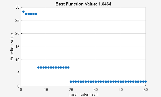
为了寻找更好的解，创建一个 MultiStart 对象。在求解器迭代时绘制最佳函数值。

ms = MultiStart(PlotFcns=@gsplotbestf);

再次调用 solve，这次使用 ms。为 MultiStart 指定 50 个起点。

rng default % For reproducibility
[sol2,fval2] = solve(prob,x0,ms,MinNumStartPoints=50)

Solving problem using MultiStart.

Figure MultiStart contains an axes object. The axes object with title Best Function Value: 1.6464, xlabel Local solver call, ylabel Function value contains an object of type scatter.

MultiStart completed the runs from all start points. 

All 50 local solver runs converged with a positive local solver exitflag.

sol2 = struct with fields:
    a: -2.9852
    b: -0.2472
    c: -0.4968
    d: -1.0438

fval2 = 
1.6464

MultiStart 在参数值 (-3,-1/4,-1/2,-1) 附近找到了一个全局解。该解等效于接近真实参数值 (-3,1/4,1/2,1) 的解，因为改变除第一个之外的所有系数的符号都会产生相同的误差数值。残差误差的范数从约 28 减少至约 1.6，减少了 10 倍以上。

另请参阅

MultiStart | solve | lsqnonlin

MultiStart 与 lsqnonlin，基于问题