使用 GlobalSearch 和 MultiStart 最大化单色偏振光干涉图案
此示例显示如何使用函数 GlobalSearch 和 MultiStart。
简介
这个例子展示了 Global Optimization Toolbox 函数,特别是 GlobalSearch 和 MultiStart,如何帮助定位电磁干涉模式的最大值。为了简化建模,模式来自从点源扩散的单色偏振光。
在点 x 和时间 t 处沿极化方向测量的源 i 产生的电场为
![]()
其中 ![]() 是源
是源 ![]() 在时间零点的相位,
在时间零点的相位,![]() 是光速,
是光速,![]() 是光的频率,
是光的频率,![]() 是源
是源 ![]() 的振幅,
的振幅,![]() 是源
是源 ![]() 到
到 ![]() 的距离。
的距离。
对于固定点 ![]() ,光的强度是净电场平方的时间平均值。净电场是所有源产生的电场的总和。时间平均值仅取决于
,光的强度是净电场平方的时间平均值。净电场是所有源产生的电场的总和。时间平均值仅取决于 ![]() 处的电场的大小和相对相位。要计算净电场,需要使用相量法将个体贡献相加。对于相量,每个源都贡献一个向量。向量的长度是振幅除以与源的距离,向量的角度
处的电场的大小和相对相位。要计算净电场,需要使用相量法将个体贡献相加。对于相量,每个源都贡献一个向量。向量的长度是振幅除以与源的距离,向量的角度 ![]() 是该点的相位。
是该点的相位。
对于这个例子,我们定义了三个具有相同频率(![]() )和振幅(
)和振幅(![]() )但初始相位不同(
)但初始相位不同(![]() )的点源。我们将这些源排列在一个固定的平面上。
)的点源。我们将这些源排列在一个固定的平面上。
% Frequency is proportional to the number of peaks
relFreqConst = 2*pi*2.5;
amp = 2.2;
phase = -[0; 0.54; 2.07];

numSources = 3;
height = 3;

% All point sources are aligned at [x_i,y_i,z]
xcoords = [2.4112
           0.2064
           1.6787];
ycoords = [0.3957
           0.3927
           0.9877];
zcoords = height*ones(numSources,1);

origins = [xcoords ycoords zcoords];
可视化干涉图样
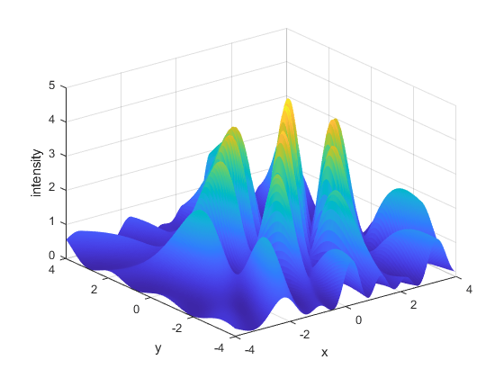
现在让我们想象一下平面 z = 0 上的干涉模式切片。
从下图可以看出,有许多峰和谷,表示建设性和破坏性干扰。
% Pass additional parameters via an anonymous function:
waveIntensity_x = @(x) waveIntensity(x,amp,phase, ...
    relFreqConst,numSources,origins);
% Generate the grid
[X,Y] = meshgrid(-4:0.035:4,-4:0.035:4);
% Compute the intensity over the grid
Z = arrayfun(@(x,y) waveIntensity_x([x y]),X,Y);
% Plot the surface and the contours
figure
surf(X,Y,Z,'EdgeColor','none')
xlabel('x')
ylabel('y')
zlabel('intensity')
提出优化问题
我们对这个波强度达到最高峰的位置感兴趣。
波强度(![]() )随着我们远离源而衰减,与
)随着我们远离源而衰减,与 ![]() 成比例。因此,让我们通过给问题添加约束来限制可行解的空间。
成比例。因此,让我们通过给问题添加约束来限制可行解的空间。
如果我们用光圈来限制光源的曝光,那么我们可以预期最大值位于光圈在我们的观察平面上的投影的交点处。我们通过将搜索限制在以每个源为中心的圆形区域来模拟光圈的影响。
我们还通过添加问题边界来限制解空间。尽管这些边界可能是多余的(考虑到非线性约束),但它们很有用,因为它们限制了生成起点的范围(有关更多信息,请参阅 GlobalSearch 和 MultiStart 的工作原理)。
现在我们的问题变成了:
![]()
约束条件为
![]()
![]()
![]()
![]()
![]()
其中 ![]() 和
和 ![]() 分别是
分别是 ![]() 点源的坐标和孔径半径。每个源都有一个半径为 3 的孔径。给定的边界涵盖了可行区域。
点源的坐标和孔径半径。每个源都有一个半径为 3 的孔径。给定的边界涵盖了可行区域。
目标(![]() )和非线性约束函数分别在单独的 MATLAB® 文件
)和非线性约束函数分别在单独的 MATLAB® 文件 waveIntensity.m 和 apertureConstraint.m 中定义,这两个文件列在本示例的末尾。
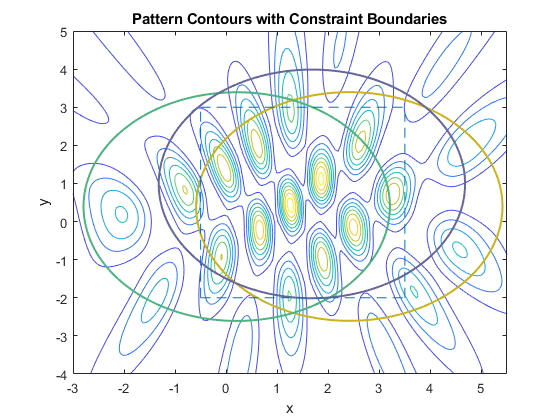
带约束的可视化
现在让我们将叠加了非线性约束边界的干涉模式的轮廓可视化。可行区域是三个圆圈(黄色、绿色和蓝色)交点的内部。变量的边界用虚线框表示。
% Visualize the contours of our interference surface
domain = [-3 5.5 -4 5];
figure;
ezcontour(@(X,Y) arrayfun(@(x,y) waveIntensity_x([x y]),X,Y),domain,150);
hold on

% Plot constraints
g1 = @(x,y)  (x-xcoords(1)).^2 + (y-ycoords(1)).^2 - 9;
g2 = @(x,y)  (x-xcoords(2)).^2 + (y-ycoords(2)).^2 - 9;
g3 = @(x,y)  (x-xcoords(3)).^2 + (y-ycoords(3)).^2 - 9;
h1 = ezplot(g1,domain);
h1.Color = [0.8 0.7 0.1]; % yellow
h1.LineWidth = 1.5;
h2 = ezplot(g2,domain);
h2.Color = [0.3 0.7 0.5]; % green
h2.LineWidth = 1.5;
h3 = ezplot(g3,domain);
h3.Color = [0.4 0.4 0.6]; % blue
h3.LineWidth = 1.5;

% Plot bounds
lb = [-0.5 -2];
ub = [3.5 3];
line([lb(1) lb(1)],[lb(2) ub(2)],'LineStyle','--')
line([ub(1) ub(1)],[lb(2) ub(2)],'LineStyle','--')
line([lb(1) ub(1)],[lb(2) lb(2)],'LineStyle','--')
line([lb(1) ub(1)],[ub(2) ub(2)],'LineStyle','--')
title('Pattern Contours with Constraint Boundaries')
使用局部求解器设置和解决问题
给定非线性约束,我们需要一个受约束的非线性求解器,即 fmincon。
让我们建立一个描述优化问题的问题结构体。我们希望最大化强度函数,因此我们对从 waveIntensity 返回的值取反。让我们选择一个恰好位于可行区域附近的任意起点。
对于这个小问题,我们将使用 fmincon 的 SQP 算法。
% Pass additional parameters via an anonymous function:
apertureConstraint_x = @(x) apertureConstraint(x,xcoords,ycoords);

% Set up fmincon's options
x0 = [3 -1];
opts = optimoptions('fmincon','Algorithm','sqp');
problem = createOptimProblem('fmincon','objective', ...
    @(x) -waveIntensity_x(x),'x0',x0,'lb',lb,'ub',ub, ...
    'nonlcon',apertureConstraint_x,'options',opts);

% Call fmincon
[xlocal,fvallocal] = fmincon(problem)
Local minimum found that satisfies the constraints.

Optimization completed because the objective function is non-decreasing in
feasible directions, to within the value of the optimality tolerance,
and constraints are satisfied to within the value of the constraint tolerance.


xlocal =

   -0.5000    0.4945


fvallocal =

   -1.4438
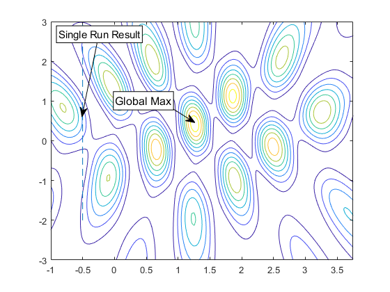
现在,让我们通过在等高线图中显示 fmincon 的结果来看看我们做得如何。请注意,fmincon 没有达到全局最大值,这也在图中进行了标注。请注意,我们将仅绘制在解中活跃的边界。
[~,maxIdx] = max(Z(:));
xmax = [X(maxIdx),Y(maxIdx)]
figure
contour(X,Y,Z)
hold on

% Show bounds
line([lb(1) lb(1)],[lb(2) ub(2)],'LineStyle','--')

% Create textarrow showing the location of xlocal
annotation('textarrow',[0.25 0.21],[0.86 0.60],'TextEdgeColor',[0 0 0],...
    'TextBackgroundColor',[1 1 1],'FontSize',11,'String',{'Single Run Result'});

% Create textarrow showing the location of xglobal
annotation('textarrow',[0.44 0.50],[0.63 0.58],'TextEdgeColor',[0 0 0],...
    'TextBackgroundColor',[1 1 1],'FontSize',12,'String',{'Global Max'});

axis([-1 3.75 -3 3])
xmax =

    1.2500    0.4450
使用 GlobalSearch 和 MultiStart
给定一个任意的初始猜测,fmincon 会停留在附近的局部最大值。Global Optimization Toolbox 求解器,特别是 GlobalSearch 和 MultiStart,为我们提供了更好的机会来找到全局最大值,因为它们将从多个生成的初始点(或者我们自己的自定义点,如果我们选择的话)尝试 fmincon。
我们的问题已经在 problem 结构体中设置好了,所以现在我们构建我们的求解器对象并运行它们。run 的第一个输出是找到的最佳结果的位置。
% Construct a GlobalSearch object
gs = GlobalSearch;
% Construct a MultiStart object based on our GlobalSearch attributes
ms = MultiStart;

rng(4,'twister') % for reproducibility

% Run GlobalSearch
tic;
[xgs,~,~,~,solsgs] = run(gs,problem);
toc
xgs

% Run MultiStart with 15 randomly generated points
tic;
[xms,~,~,~,solsms] = run(ms,problem,15);
toc
xms
GlobalSearch stopped because it analyzed all the trial points.

All 14 local solver runs converged with a positive local solver exit flag.
Elapsed time is 0.229525 seconds.

xgs =

    1.2592    0.4284


MultiStart completed the runs from all start points.

All 15 local solver runs converged with a positive local solver exit flag.
Elapsed time is 0.109984 seconds.

xms =

    1.2592    0.4284
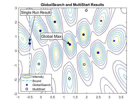
检查结果
让我们检查一下两个求解器返回的结果。需要注意的一件重要事情是,结果将根据为每个求解器创建的随机起点而有所不同。再次运行此示例可能会得出不同的结果。将最佳结果 xgs 和 xms 的坐标打印到命令行。我们将展示由 GlobalSearch 和 MultiStart 返回的独特结果,并强调每个求解器在与全局解的接近程度方面的最佳结果。
每个求解器的第五个输出是一个包含找到的不同极小值(或在本例中极大值)的向量。我们将根据之前使用的轮廓图绘制结果的 (x,y) 对 solsgs 和 solsms。
% Plot GlobalSearch results using the '*' marker
xGS = cell2mat({solsgs(:).X}');
scatter(xGS(:,1),xGS(:,2),'*','MarkerEdgeColor',[0 0 1],'LineWidth',1.25)

% Plot MultiStart results using a circle marker
xMS = cell2mat({solsms(:).X}');
scatter(xMS(:,1),xMS(:,2),'o','MarkerEdgeColor',[0 0 0],'LineWidth',1.25)
legend('Intensity','Bound','GlobalSearch','MultiStart','Location','best')

title('GlobalSearch and MultiStart Results')
放宽界限
对问题采样严格的边界,GlobalSearch 和 MultiStart 都能够在这次运行中找到全局最大值。
在实践中,当对目标函数或约束了解不多时,找到严格的边界可能很困难。但一般来说,我们可能能够猜出一个我们想要限制起点集的合理区域。为了说明目的,让我们放宽边界来定义一个更大的区域来生成起点并重新尝试求解器。
% Relax the bounds to spread out the start points
problem.lb = -5*ones(2,1);
problem.ub = 5*ones(2,1);

% Run GlobalSearch
tic;
[xgs,~,~,~,solsgs] = run(gs,problem);
toc
xgs

% Run MultiStart with 15 randomly generated points
tic;
[xms,~,~,~,solsms] = run(ms,problem,15);
toc
xms
GlobalSearch stopped because it analyzed all the trial points.

All 4 local solver runs converged with a positive local solver exit flag.
Elapsed time is 0.173760 seconds.

xgs =

    0.6571   -0.2096


MultiStart completed the runs from all start points.

All 15 local solver runs converged with a positive local solver exit flag.
Elapsed time is 0.134150 seconds.

xms =

    2.4947   -0.1439
% Show the contours
figure
contour(X,Y,Z)
hold on

% Create textarrow showing the location of xglobal
annotation('textarrow',[0.44 0.50],[0.63 0.58],'TextEdgeColor',[0 0 0],...
    'TextBackgroundColor',[1 1 1],'FontSize',12,'String',{'Global Max'});
axis([-1 3.75 -3 3])

% Plot GlobalSearch results using the '*' marker
xGS = cell2mat({solsgs(:).X}');
scatter(xGS(:,1),xGS(:,2),'*','MarkerEdgeColor',[0 0 1],'LineWidth',1.25)

% Plot MultiStart results using a circle marker
xMS = cell2mat({solsms(:).X}');
scatter(xMS(:,1),xMS(:,2),'o','MarkerEdgeColor',[0 0 0],'LineWidth',1.25)

% Highlight the best results from each:
% GlobalSearch result in red, MultiStart result in blue
plot(xgs(1),xgs(2),'sb','MarkerSize',12,'MarkerFaceColor',[1 0 0])
plot(xms(1),xms(2),'sb','MarkerSize',12,'MarkerFaceColor',[0 0 1])
legend('Intensity','GlobalSearch','MultiStart','Best GS','Best MS','Location','best')

title('GlobalSearch and MultiStart Results with Relaxed Bounds')
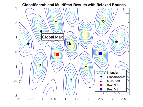
GlobalSearch 的最佳结果用红色方块表示,MultiStart 的最佳结果用蓝色方块表示。
调整 GlobalSearch 参数
请注意,在这次运行中,由于边界定义的区域较大,所以两个求解器都无法识别最大强度的点。我们可以尝试用几种方法来克服这个问题。首先,我们来检查 GlobalSearch。
请注意,GlobalSearch 仅运行了 fmincon 几次。为了增加找到全局最大值的机会,我们想运行更多的点。为了将起点集限制为最有可能找到全局最大值的候选点,我们将通过将 StartPointsToRun 属性设置为 bounds-ineqs 来指示每个求解器忽略不满足约束的起点。此外,我们将设置 MaxWaitCycle 和 BasinRadiusFactor 属性,以便 GlobalSearch 能够快速识别窄峰。减少 MaxWaitCycle 会导致 GlobalSearch 以比默认设置更频繁的 BasinRadiusFactor 频率减少吸引盆半径。
% Increase the total candidate points, but filter out the infeasible ones
gs = GlobalSearch(gs,'StartPointsToRun','bounds-ineqs', ...
    'MaxWaitCycle',3,'BasinRadiusFactor',0.3);
% Run GlobalSearch
tic;
xgs = run(gs,problem);
toc
xgs
GlobalSearch stopped because it analyzed all the trial points.

All 10 local solver runs converged with a positive local solver exit flag.
Elapsed time is 0.242955 seconds.

xgs =

    1.2592    0.4284
利用 MultiStart 的并行功能
提高找到全局最大值的机会的一种强力方法就是尝试更多的起点。再次强调,这可能并不适用于所有情况。在我们的案例中,到目前为止我们只尝试了一小组,并且运行时间也不是很长。因此,尝试更多的起点是合理的。为了加快计算速度,如果 Parallel Computing Toolbox™ 可用,我们将并行运行 MultiStart。
% Set the UseParallel property of MultiStart
ms = MultiStart(ms,'UseParallel',true);

try
    demoOpenedPool = false;
    % Create a parallel pool if one does not already exist
    % (requires Parallel Computing Toolbox)
    if max(size(gcp)) == 0 % if no pool
        parpool
        demoOpenedPool = true;
    end
catch ME
    warning(message('globaloptim:globaloptimdemos:opticalInterferenceDemo:noPCT'));
end

% Run the solver
tic;
xms = run(ms,problem,100);
toc
xms

if demoOpenedPool
    % Make sure to delete the pool if one was created in this example
    delete(gcp) % delete the pool
end
MultiStart completed the runs from all start points.

All 100 local solver runs converged with a positive local solver exit flag.
Elapsed time is 0.956671 seconds.

xms =

    1.2592    0.4284
目标和非线性约束
这里我们列出了定义优化问题的函数:
function p = waveIntensity(x,amp,phase,relFreqConst,numSources,origins)
% WaveIntensity Intensity function for opticalInterferenceDemo.

%   Copyright 2009 The MathWorks, Inc.

d = distanceFromSource(x,numSources,origins);
ampVec = [sum(amp./d .* cos(phase - d*relFreqConst));
    sum(amp./d .* sin(phase - d*relFreqConst))];

% Intensity is ||AmpVec||^2
p = ampVec'*ampVec;
function [c,ceq] = apertureConstraint(x,xcoords,ycoords)
% apertureConstraint Aperture constraint function for opticalInterferenceDemo.

%   Copyright 2009 The MathWorks, Inc.

ceq = [];
c = (x(1) - xcoords).^2 + (x(2) - ycoords).^2 - 9;
function d = distanceFromSource(v,numSources,origins)
% distanceFromSource Distance function for opticalInterferenceDemo.

%   Copyright 2009 The MathWorks, Inc.

d = zeros(numSources,1);
for k = 1:numSources
    d(k) = norm(origins(k,:) - [v 0]);
end