种群多样性
种群多样性的重要性
决定遗传算法性能的最重要因素之一是种群的多样性。如果个体之间的平均距离较大,则多样性较高;如果平均距离较小,则多样性较低。获得适当数量的多样性需要一个反复试验的过程。如果多样性太高或太低,遗传算法可能不会表现良好。
本节说明如何通过设定种群的初始范围来控制多样性。变异和交叉 中的主题“设置突变量”描述了变异如何影响多样性。
本节还解释了如何设置种群规模。
设置初始范围
默认情况下,ga 使用创建函数创建一个随机初始种群。您可以在 InitialPopulationRange 选项中指定初始种群中向量的范围。
注意:初始范围通过指定下界和上界来限制初始种群中点的范围。后续生成可以包含其条目不位于初始范围内的点。使用 lb 和 ub 输入参量为所有代设置上界和下界。
如果您大概知道问题的解在哪里,请指定初始范围,以便它包含您对解的猜测。然而,如果种群具有足够的多样性,遗传算法即使不在初始范围内也能找到解。
这个例子说明了初始范围如何影响遗传算法的性能。该示例使用了拉斯特里金函数,在 最小化拉斯特里金函数 中进行了描述。函数的最小值为 0,出现在原点。
rng(1) % For reproducibility
fun = @rastriginsfcn;
nvar = 2;
options = optimoptions('ga','PlotFcn',{'gaplotbestf','gaplotdistance'},...
    'InitialPopulationRange',[1;1.1]);
[x,fval] = ga(fun,nvar,[],[],[],[],[],[],[],options)
ga stopped because the average change in the fitness value is less than options.FunctionTolerance.
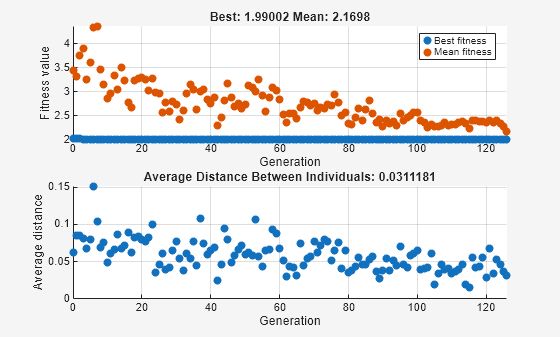
x = 1×2

    0.9942    0.9950
fval =
1.9900
上图显示的是每代的最佳适应度,表明适应度值的降低进展不大。下图显示的是每代个体之间的平均距离,这是衡量种群多样性的一个很好的指标。对于此初始范围的设置,多样性太少,算法无法取得进展。
接下来,尝试将 InitialPopulationRange 设置为 [1;100]。这次的结果更加变数。当前随机数设置会导致相当典型的结果。
options.InitialPopulationRange = [1;100];
[x,fval] = ga(fun,nvar,[],[],[],[],[],[],[],options)
ga stopped because the average change in the fitness value is less than options.FunctionTolerance.
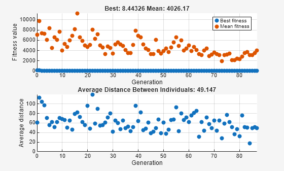
x = 1×2

   -2.1352   -0.0497
fval =
8.4433
这次,遗传算法取得了进展,但是由于个体之间的平均距离太大,导致最佳个体距离最优解还很远。
现在将 InitialPopulationRange 设置为 [1;2]。此设置非常适合解决这个问题。
options.InitialPopulationRange = [1;2];
[x,fval] = ga(fun,nvar,[],[],[],[],[],[],[],options)
ga stopped because it exceeded options.MaxGenerations.
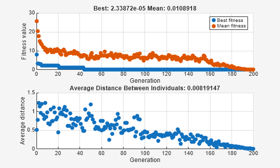
x = 1×2
10-3 ×

    0.2473   -0.2382
fval =
2.3387e-05
适当的多样性通常使得 ga 返回比前两种情况更好的结果。
ga 中的自定义绘图函数和线性约束
此示例显示了 @gacreationlinearfeasible(线性约束问题的默认创建函数)如何为 ga 创建种群。种群分散性较好,且偏向于位于约束边界上。该示例使用自定义绘图函数。
适应度函数
适应度函数是 lincontest6,运行此示例时可用。lincontest6 是两个变量的二次函数:
![]()
自定义绘图函数
将以下代码保存到 MATLAB® 路径上名为 gaplotshowpopulation2 的文件中。
function state = gaplotshowpopulation2(~,state,flag,fcn)
%gaplotshowpopulation2 Plots the population and linear constraints in 2-d.
%   STATE = gaplotshowpopulation2(OPTIONS,STATE,FLAG) plots the population
%   in two dimensions.
%
%   Example:
%     fun = @lincontest6;
%     options = gaoptimset('PlotFcn',{{@gaplotshowpopulation2,fun}});
%     [x,fval,exitflag] = ga(fun,2,A,b,[],[],lb,[],[],options);

% This plot function works in 2-d only
if size(state.Population,2) > 2
    return;
end
if nargin < 4
    fcn = [];
end
% Dimensions to plot
dimensionsToPlot = [1 2];

switch flag
    % Plot initialization
    case 'init'
        pop = state.Population(:,dimensionsToPlot);
        plotHandle = plot(pop(:,1),pop(:,2),'*');
        set(plotHandle,'Tag','gaplotshowpopulation2')
        title('Population plot in two dimension','interp','none')
        xlabelStr = sprintf('%s %s','Variable ', num2str(dimensionsToPlot(1)));
        ylabelStr = sprintf('%s %s','Variable ', num2str(dimensionsToPlot(2)));
        xlabel(xlabelStr,'interp','none');
        ylabel(ylabelStr,'interp','none');
        hold on;

        % plot the inequalities
        plot([0 1.5],[2 0.5],'m-.') %  x1 + x2 <= 2
        plot([0 1.5],[1 3.5/2],'m-.'); % -x1 + 2*x2 <= 2
        plot([0 1.5],[3 0],'m-.'); % 2*x1 + x2 <= 3
        % plot lower bounds
        plot([0 0], [0 2],'m-.'); % lb = [ 0 0];
        plot([0 1.5], [0 0],'m-.'); % lb = [ 0 0];
        set(gca,'xlim',[-0.7,2.2])
        set(gca,'ylim',[-0.7,2.7])
        axx = gcf;
        % Contour plot the objective function
        if ~isempty(fcn)
            range = [-0.5,2;-0.5,2];
            pts = 100;
            span = diff(range')/(pts - 1);
            x = range(1,1): span(1) : range(1,2);
            y = range(2,1): span(2) : range(2,2);

            pop = zeros(pts * pts,2);
            values = zeros(pts,1);
            k = 1;
            for i = 1:pts
                for j = 1:pts
                    pop(k,:) = [x(i),y(j)];
                    values(k) = fcn(pop(k,:));
                    k = k + 1;
                end
            end
            values = reshape(values,pts,pts);
            contour(x,y,values);
            colorbar
        end
        % Show the initial population
        ax = gca;
        fig = figure;
        copyobj(ax,fig);colorbar
        % Pause for three seconds to view the initial plot, then resume
        figure(axx)
        pause(3);
    case 'iter'
        pop = state.Population(:,dimensionsToPlot);
        plotHandle = findobj(get(gca,'Children'),'Tag','gaplotshowpopulation2');
        set(plotHandle,'Xdata',pop(:,1),'Ydata',pop(:,2));
end
自定义绘图函数绘制表示线性不等式和边界的约束,绘制适应度函数的水平曲线,并绘制种群演变过程。该绘图函数不仅需要有通常的输入 (options,state,flag),还需要有适应度函数的函数句柄,在本例中为 @lincontest6。为了生成水平曲线,自定义绘图函数需要适应度函数。
问题约束
包括边界和线性约束。
A = [1,1;-1,2;2,1];
b = [2;2;3];
lb = zeros(2,1);
包含绘图函数的选项
设置选项以在 ga 运行时包含绘图函数。
options = optimoptions('ga','PlotFcns',...
{{@gaplotshowpopulation2,@lincontest6}});
运行问题并观察种群
在第一个图中,初始种群在线性约束边界上有许多成员。种群的分散度较为合理。
rng default % for reproducibility
[x,fval] = ga(@lincontest6,2,A,b,[],[],lb,[],[],options);
ga stopped because the average change in the fitness value is less than options.FunctionTolerance.
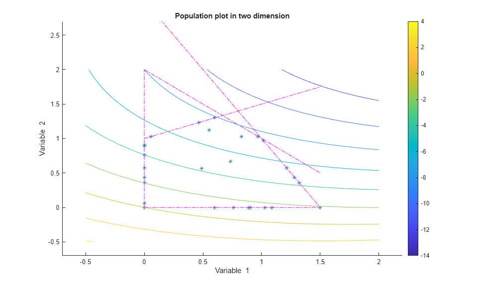

ga 快速收敛到一个点,即解。
设置种群大小
Population 选项中的 Population size 字段决定了每代种群的大小。增加种群规模可以使遗传算法搜索更多的点,从而获得更好的结果。然而,种群规模越大,遗传算法计算每代所需的时间就越长。
注意
您应该将种群规模设置为至少变量数量的值,以便每个种群中的个体跨越被搜索的空间。
您可以尝试使用不同的种群大小设置来获得良好的结果,而无需花费过多的运行时间。