Lane Detection
This example shows how to implement a lane-marking detection algorithm for FPGAs.
Lane detection is a critical processing stage in Advanced Driving Assistance Systems (ADAS). Automatically detecting lane boundaries from a video stream is computationally challenging and therefore hardware accelerators such as FPGAs and GPUs are often required to achieve real time performance.
In this example model, an FPGA-based lane candidate generator is coupled with a software-based polynomial fitting engine, to determine lane boundaries.
Download Input File
This example uses the visionhdl_caltech.avi file as an input. The file is approximately 19 MB in size. Download the file from the MathWorks® website and unzip the downloaded file.
laneZipFile = matlab.internal.examples.downloadSupportFile('visionhdl_hdlcoder','caltech_dataset.zip');
[outputFolder,~,~] = fileparts(laneZipFile);
unzip(laneZipFile,outputFolder);
caltechVideoFile = fullfile(outputFolder,'caltech_dataset');
addpath(caltechVideoFile);
System Overview
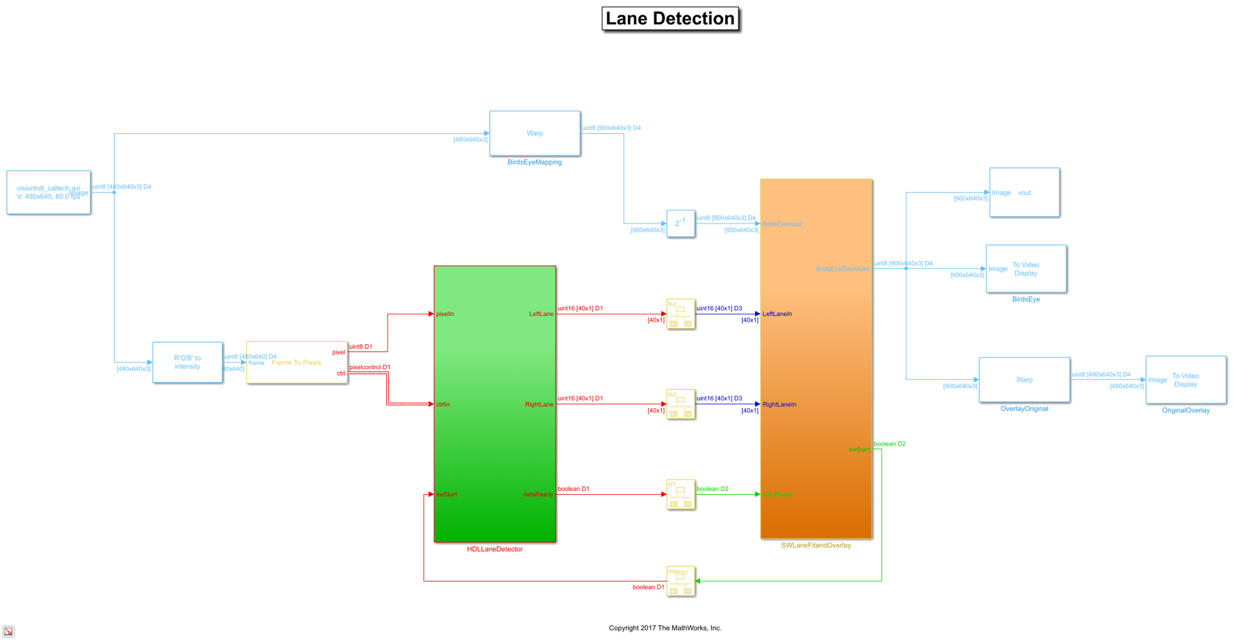
The LaneDetectionHDL.slx system is shown below. The HDLLaneDetector subsystem represents the hardware accelerated part of the design, while the SWLaneFitandOverlay subsystem represent the software based polynomial fitting engine. Prior to the Frame To Pixels (Vision HDL Toolbox) block, the RGB input is converted to intensity color space.
modelname = 'LaneDetectionHDL';
open_system(modelname);
set_param(modelname,'SampleTimeColors','on');
set_param(modelname,'SimulationCommand','Update');
set_param(modelname,'Open','on');
set(allchild(0),'Visible','off');
HDL Lane Detector
The HDL Lane Detector represents the hardware-accelerated part of the design. This subsystem receives the input pixel stream from the front-facing camera source, transforms the view to obtain the birds-eye view, locates lane marking candidates from the transformed view and then buffers them up into a vector to send to the software side for curve fitting and overlay.
set_param(modelname, 'SampleTimeColors', 'off');
open_system([modelname '/HDLLaneDetector'],'force');

Birds-Eye View
The Birds-Eye View (Vision HDL Toolbox) block transforms the front-facing camera view to a birds-eye perspective. Working with the images in this view simplifies the processing requirements of the downstream lane detection algorithms. The front-facing view suffers from perspective distortion, causing the lanes to converge at the vanishing point. The perspective distortion is corrected by applying an inverse perspective transform.
The Inverse Perspective Mapping (IPM) is given by the following expression:

The homography matrix, h, is derived from four intrinsic parameters of the physical camera setup, namely the focal length, pitch, height, and principle point (from a pinhole camera model).
You can estimate the homography matrix by using the Computer Vision Toolbox™ estgeotform2d function or the Image Processing Toolbox™ fitgeotform2d function to create a projtform2d object. These functions require a set of matched points between the source frame and birds-eye view frame. The source frame points are taken as the vertices of a trapezoidal region of interest, and can extend past the source frame limits to capture a larger region. For the trapezoid shown the point mapping is:
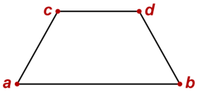
![$$sourcePoints = [c_{x},c_{y};\ d_{x},d_{y};\ a_{x},a_{y};\ b_{x},b_{y}]$$](../../examples/visionhdl_hdlcoder/win64/LaneDetectionHDLExample_eq15520422000910455757.png)
![$$birdsEyePoints = [1,1;\ bAPPL,1;\ 1,bAVL;\ bAPPL,bAVL]$$](../../examples/visionhdl_hdlcoder/win64/LaneDetectionHDLExample_eq11628490074344606081.png)
Where bAPPL and bAVL are the birds-eye view active pixels per line and active video lines respectively.
Direct evaluation of the source (front-facing) to destination (birds-eye) mapping in real time on FPGA/ASIC hardware is challenging. The requirement for division along with the potential for non-sequential memory access from a frame buffer mean that the computational requirements of this part of the design are substantial. Therefore instead of directly evaluating the IPM calculation in real time, an offline analysis of the input to output mapping has been performed and used to pre-compute a mapping scheme. This is possible as the homography matrix is fixed after factory calibration/installation of the camera, due to the camera position, height and pitch being fixed.
In this particular example, the birds-eye output image is a frame of [700x640] dimensions, whereas the front-facing input image is of [480x640] dimensions. There is not sufficient blanking available in order to output the full birds-eye frame before the next front-facing camera input is streamed in. The Birds-Eye View block does not accept any new frame data until it has finished processing the current birds-eye frame.
open_system([modelname '/HDLLaneDetector'],'force');
Line Buffering and Address Computation
A full sized projective transformation from input to output would result in a [900x640] output image. This requires that the full [480x640] input image is stored in memory, while the source pixel location is calculated using the source location and homography matrix. Ideally on-chip memory should be used for this purpose, removing the requirement for an off-chip frame buffer.
You can determine the number of lines to buffer on-chip by performing inverse row mapping using the homography matrix. The following script calculates the homography matrix from the point mapping, using it to an inverse transform to map the source frame rows to birds-eye view rows.
% Source & Birds-Eye Frame Parameters
%   AVL:  Active Video Lines, APPL: Active Pixels Per Line
sAVL  = 480;
sAPPL = 640;
% Birds-Eye Frame
bAVL  = 700;
bAPPL = 640;
% Determine Homography Matrix
%   Point Mapping [NW; NE; SW; SE]
sourcePoints   = [218,196; 421,196; -629,405; 1276,405];
birdsEyePoints = [001,001; 640,001;  001,900;  640,900];
%   Estimate Transform
tf = estgeotform2d(sourcePoints,birdsEyePoints,'projective');
%   Homography Matrix
h = tf.T;
% Visualize Birds-Eye ROI on Source Frame
vidObj   = VideoReader('visionhdl_caltech.avi');
vidFrame = readFrame(vidObj);
vidFrameAnnotated = insertShape(vidFrame,'Polygon',[sourcePoints(1,:) ...
    sourcePoints(2,:) sourcePoints(4,:) sourcePoints(3,:)],           ...
    'LineWidth',5,'Color','red');
vidFrameAnnotated = insertShape(vidFrameAnnotated,'FilledPolygon',    ...
    [sourcePoints(1,:) sourcePoints(2,:) sourcePoints(4,:)            ...
    sourcePoints(3,:)],'LineWidth',5,'Color','red','Opacity',0.2);
figure(1);
subplot(2,1,1);
imshow(vidFrameAnnotated)
title('Source Video Frame');
% Determine Required Birds-Eye Line Buffer Depth
%   Inverse Row Mapping at Frame Centre
x = round(sourcePoints(2,1)-((sourcePoints(2,1)-sourcePoints(1,1))/2));
Y = zeros(1,bAVL);
for ii = 1:1:bAVL
    [~,Y(ii)] = transformPointsInverse(tf,x,ii);
end
numRequiredRows = ceil(Y(0.98*bAVL) - Y(1));
% Visualize Inverse Row Mapping
subplot(2,1,2);
plot(Y,'HandleVisibility','off');   % Inverse Row Mapping
xline(0.98*bAVL,'r','98%','LabelHorizontalAlignment','left',          ...
    'HandleVisibility','off');      % Line Buffer Depth
yline(Y(1),'r--','HandleVisibility','off')
yline(Y(0.98*bAVL),'r')
title('Birds-Eye View Inverse Row Mapping');
xlabel('Output Row');
ylabel('Input Row');
legend(['Line Buffer Depth: ',num2str(numRequiredRows),' lines'],     ...
    'Location','northwest');
axis equal;
grid on;

The plot shows the mapping of input line to output line revealing that in order to generate the first 700 lines of the top down birds eye output image, around 50 lines of the input image are required. This is an acceptable number of lines to store using on-chip memory.
Lane Detection
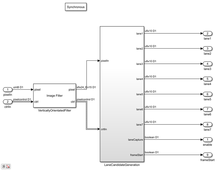
With the birds-eye view image obtained, the actual lane detection can be performed. There are many techniques which can be considered for this purpose. To achieve an implementation which is robust, works well on streaming image data and which can be implemented in FPGA/ASIC hardware at reasonable resource cost, this example uses the approach described in [1]. This algorithm performs a full image convolution with a vertically oriented first order Gaussian derivative filter kernel, followed by sub-region processing.
open_system([modelname '/HDLLaneDetector/LaneDetection'],'force');
Vertically Oriented Filter Convolution
Immediately following the birds-eye mapping of the input image, the output is convolved with a filter designed to locate strips of high intensity pixels on a dark background. The width of the kernel is 8 pixels, which relates to the width of the lines that appear in the birds-eye image. The height is set to 16 which relates to the size of the dashed lane markings which appear in the image. As the birds-eye image is physically related to the height, pitch etc. of the camera, the width at which lanes appear in this image is intrinsically related to the physical measurement on the road. The width and height of the kernel may need to be updated when operating the lane detection system in different countries.
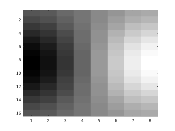
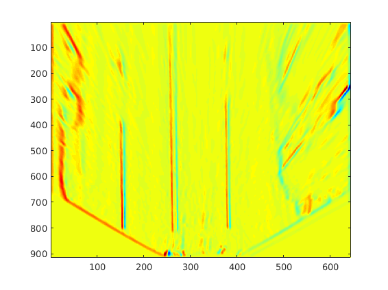
The output of the filter kernel is shown below, using jet colormap to highlight differences in intensity. Because the filter kernel is a general, vertically oriented Gaussian derivative, there is some response from many different regions. However, for the locations where a lane marking is present, there is a strong positive response located next to a strong negative response, which is consistent across columns. This characteristic of the filter output is used in the next stage of the detection algorithm to locate valid lane candidates.
Lane Candidate Generation
After convolution with the Gaussian derivative kernel, sub-region processing of the output is performed in order to find the coordinates where a lane marking is present. Each region consists of 18 lines, with a ping-pong memory scheme in place to ensure that data can be continuously streamed through the subsystem.
%Seeing as
open_system([modelname '/HDLLaneDetector/LaneDetection/LaneCandidateGeneration'],'force');

Histogram Column Count
Firstly, the HistogramColumnCount subsystem counts the number of thresholded pixels in each column over the 18 line region. A high column count indicates that a lane is likely present in the region. This count is performed for both the positive and the negative thresholded images. The positive histogram counts are offset to account for the kernel width. Lane candidates occur where the positive count and negative counts are both high. This exploits the previously noted property of the convolution output where positive tracks appear next to negative tracks.
Internally, the column counting histogram generates the control signaling that selects an 18 line region, computes the column histogram, and outputs the result when ready. A ping-pong buffering scheme is in place which allows one histogram to be reading while the next is writing.
Overlap and Multiply
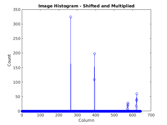
As noted, when a lane is present in the birds-eye image, the convolution result will produce strips of high-intensity positive output located next to strips of high-intensity negative output. The positive and negative column count histograms locate such regions. In order to amplify these locations, the positive count output is delayed by 8 clock cycles (an intrinsic parameter related to the kernel width), and the positive and negative counts are multiplied together. This amplifies columns where the positive and negative counts are in agreement, and minimizes regions where there is disagreement between the positive and negative counts. The design is pipelined in order to ensure high throughput operation.
Zero Crossing Filter
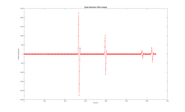
At the output of the Overlap and Multiply subsystem, peaks appear where there are lane markings present. A peak detection algorithm determines the columns where lane markings are present. Because the SNR is relatively high in the data, this example uses a simple FIR filtering operation followed by zero crossing detection. The Zero Crossing Filter is implemented using the Discrete FIR Filter block. It is pipelined for high-throughput operation.
Store Dominant Lanes
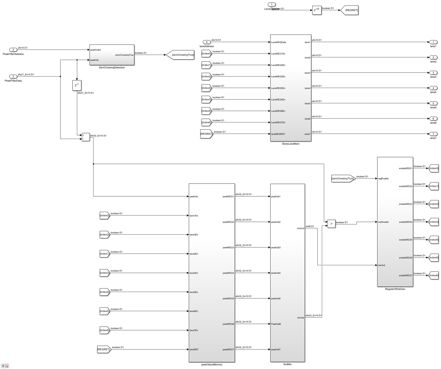
The zero crossing filter output is then passed into the Store Dominant Lanes subsystem. This subsystem has a maximum memory of 7 entries, and is reset every time a new batch of 18 lines is reached. Therefore, for each sub-region 7 potential lane candidates are generated. In this subsystem, the Zero Crossing Filter output is streamed through, and examined for potential zero crossings. If a zero crossing does occur, then the difference between the address immediately prior to zero crossing and the address after zero crossing is taken in order to get a measurement of the size of the peak. The subsystem stores the zero crossing locations with the highest magnitude.
open_system([modelname '/HDLLaneDetector/LaneDetection/LaneCandidateGeneration/StoreDominantLanes'],'force');
Compute Ego Lanes
The Lane Detection subsystem outputs the 7 most viable lane markings. In many applications, we are most interested in the lane markings that contain the lane in which the vehicle is driving. By computing the so-called "Ego-Lanes" on the hardware side of the design, we can reduce the memory bandwidth between hardware and software, by sending 2 lanes rather than 7 to the processor. The Ego-Lane computation is split into two subsystems. The FirstPassEgoLane subsystem assumes that the center column of the image corresponds to the middle of the lane, when the vehicle is correctly operating within the lane boundaries. The lane candidates which are closest to the center are therefore assumed as the ego lanes. The Outlier Removal subsystem maintains an average width of the distance from lane markings to center coordinate. Lane markers which are not within tolerance of the current width are rejected. Performing early rejection of lane markers gives better results when performing curve fitting later on in the design.
open_system([modelname '/HDLLaneDetector/ComputeEgoLanes'],'force');

Control Interface
Finally, the computed ego lanes are sent to the CtrlInterface MATLAB Function block. This state machine uses the four control signal inputs - enable, hwStart, hwDone, and swStart to determine when to start buffering, accept new lane coordinate into the 40x1 buffer and finally indicate to the software that all 40 lane coordinates have been buffered and so the lane fitting and overlay can be performed. The dataReady signal ensures that software will not attempt lane fitting until all 40 coordinates have been buffered, while the swStart signal ensures that the current set of 40 coordinates will be held until lane fitting is completed.
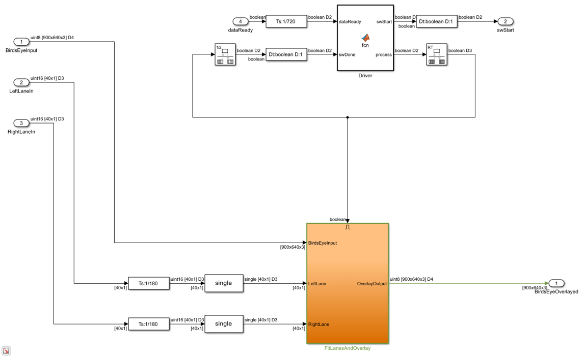
Software Lane Fit and Overlay
The detected ego-lanes are then passed to the SW Lane Fit and Overlay subsystem, where robust curve fitting and overlay is performed. Recall that the birds-eye output is produced once every two frames or so rather than on every consecutive frame. The curve fitting and overlay is therefore placed in an enabled subsystem, which is only enabled when new ego lanes are produced.
open_system([modelname '/SWLaneFitandOverlay'],'force');
Driver
The Driver MATLAB Function block controls the synchronization between hardware and software. Initially it is in a polling state, where it samples the dataReady input at regular intervals per frame to determine when hardware has buffered a full [40x1] vector of lane coordinates. Once this occurs, it transitions into software processing state where swStart and process outputs are held high. The Driver remains in the software processing state until swDone input is high. Seeing as the process output loops back to swDone input with a rate transition block in between, there is effectively a constant time budget specified for the FitLanesandOverlay subsystem to perform the fitting and overlay. When swDone is high, the Driver transitions into a synchronization state, where swStart is held low to indicate to hardware that processing is complete. The synchronization between software and hardware is such that hardware will hold the [40x1] vector of lane coordinates until the swStart signal transitions back to low. When this occurs, dataReady output of hardware will then transition back to low.
Fit Lanes and Overlay
The Fit Lanes and Overlay subsystem is enabled by the Driver. It performs the necessary arithmetic required in order to fit a polynomial onto the lane coordinate data received at input, and then draws the fitted lane and lane coordinates onto the birds-eye image.
Fit Lanes
The Fit Lanes subsystem runs a RANSAC based line-fitting routine on the generated lane candidates. RANSAC is an iterative algorithm which builds up a table of inliers based on a distance measure between the proposed curve, and the input data. At the output of this subsystem, there is a [3x1] vector which specifies the polynomial coefficients found by the RANSAC routine.
Overlay Lane Markings
The Overlay Lane Markings subsystem performs image visualization operations. It overlays the ego lanes and curves found by the lane-fitting routine.
open_system([modelname '/SWLaneFitandOverlay/FitLanesAndOverlay'],'force');

Results of the Simulation
The model includes two video displays shown at the output of the simulation results. The BirdsEye display shows the output in the warped perspective after lane candidates have been overlaid, polynomial fitting has been performed and the resulting polynomial overlaid onto the image. The OriginalOverlay display shows the BirdsEye output warped back into the original perspective.
Due to the large frame sizes used in this model, simulation can take a relatively long time to complete. If you have an HDL Verifier™ license, you can accelerate simulation speed by directly running the HDL Lane Detector subsystem in hardware using FPGA-in-the-Loop.


HDL Code Generation
To check and generate the HDL code referenced in this example, you must have an HDL Coder™ license.
To generate the HDL code, use the following command.
makehdl('LaneDetectionHDL/HDLLaneDetector')
To generate the test bench, use the following command. Note that test bench generation takes a long time due to the large data size. You may want to reduce the simulation time before generating the test bench.
makehdltb('LaneDetectionHDL/HDLLaneDetector')
For faster test bench simulation, you can generate a SystemVerilog DPIC test bench using the following command.
makehdltb('LaneDetectionHDL/HDLLaneDetector','GenerateSVDPITestBench','ModelSim')
Conclusion
This example has provided insight into the challenges of designing ADAS systems in general, with particular emphasis paid to the acceleration of critical parts of the design in hardware.
References
[1] R. K. Satzoda and Mohan M. Trivedi, "Vision based Lane Analysis: Exploration of Issues and Approaches for Embedded Realization", 2013 IEEE Conference on Computer Vision and Pattern Recognition.
[2] Video from Caltech Lanes Dataset - Mohamed Aly, "Real time Detection of Lane Markers in Urban Streets", 2008 IEEE Intelligent Vehicles Symposium - used with permission.