Main Content

RespConfig

Options for step or impulse responses

Since R2023a

Description

Use a RespConfig object to specify options for the step and impulse responses.

The step function applies this configuration as follows.

  • In the SISO case

    u(t)={U,t<T0+TdU+dU,tT0+Td.

  • In the MIMO case, the step response of the jth input channel is obtained by setting

    u(t)={U,t<T0+TdU+dUj*ej,tT0+Td,

    where ej is the jth basis vector.

The impulse function applies this configuration as follows.

u(t)=U+dU*δ(t(T0+Td))

Here:

  • U is the input signal offset.

  • dU is the input level change relative to U.

  • T0 is the start time.

  • Td is the time at which the change occurs relative to T0.

Creation

Description

example

respOpt = RespConfig creates a response configuration object with default property values.

example

respOpt = RespConfig(Name=Value) creates a response configuration object and sets its properties using one or more name-value arguments.

Properties

expand all

Input signal offset level, specified as a scalar or vector.

  • For single-input systems, InputOffset is a scalar value.

  • For multi-input systems, InputOffset is a vector of length Nu, where Nu is the number of input channels. Each vector value corresponds to the signal offset in that input channel. The functions compute the responses one input channel at a time.

  • For state-space models with offsets, set InputOffset = 'u0' to apply the step or impulse change relative to the model offsets u0, u0(t) of the LTV model, or u0(t,p) of the LPV model. For LTV and LPV models, this is the u0 output of the data function. The total input signal is then u0 + u(t).

Input level change relative to the input signal offset, specified as a scalar or vector.

  • For single-input systems, Amplitude is a scalar value.

  • For multi-input systems, Amplitude is a vector of length Nu, where Nu is the number of input channels. Each vector value corresponds to the level change amplitude in that input channel. The functions compute the responses one input channel at a time.

Input signal delay, specified as a nonnegative scalar value. This value specifies when the change occurs relative to the simulation start time T0.

Initial state values, specified as a vector or initialCondition object.

By default, the simulation starts from the steady-state condition obtained for a constant input level equal to the input offset U. For state-space models without internal delays, the initial state xinit is obtained by solving:

  • Continuous time — 0 = Axinit + BU

  • Discrete time — xinit = Axinit + BU

To start the simulation from a different initial state, use one of the following.

  • For state-space models, InitialState is a vector of length Nx, where Nx is the number of states.

  • For state-space models with offsets, you can also set InitialState to 'x0'. This uses the state offset value x0 for state-space models, x0(T0) for LTV models, or x0(T0,p(T0)) for LPV models. For LTV and LPV models, the state offset value is the x0 output of the data function evaluated at t = T0.

  • For identified LTI models, such as idtf, idss, idproc, idpoly, and idgrey models, you can use an initialCondition object to specify the initial state. Using identified models requires System Identification Toolbox™ software.

Initial parameter values for LPV models, specified as a scalar or vector.

This property is required only when you specify InputOffset = 'u0' or InitialState = [] or 'x0'. Otherwise, this value is ignored.

Object Functions

impulseImpulse response plot of dynamic system; impulse response data
stepStep response of dynamic system

Examples

collapse all

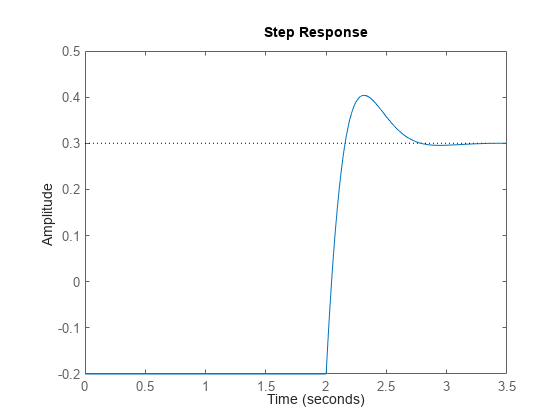
Create a transfer function model.

sys = tf([1 5],[1 10 50]);

Create an option set to specify step input offset, amplitude, and delay.

Config = RespConfig('InputOffset',-2,'Amplitude',5,'Delay',2);

Calculate the step response using the specified options.

step(sys,Config)

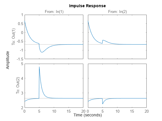
Create a state-space model.

A = [-0.8429,-0.2134;-0.5162,-1.2139];
B = [0.7254,0.7147;0,-0.2050];
C = [-0.1241,1.4090;1.4897,1.4172];
D = [0.6715,0.7172;-1.2075,0];
sys = ss(A,B,C,D);

Create a default option set and use the dot notation to specify values.

respOpt = RespConfig;
respOpt.InputOffset = [-2,3];
respOpt.Amplitude = [2,-0.5];
respOpt.InitialState = [0.1,-0.1];
respOpt.Delay = 5;

Compute the impulse response.

t = 0:0.1:20;
impulse(sys,t,respOpt)

This example shows how to apply a step change to a state-space model relative to its model offsets.

Create a random state-space model with offsets.

rng(0)
sys = rss(3,2,1); 
xoff = randn(3,1);
sys.Offsets = struct('x',xoff,'u',2,'y',[1;-1]);

Create a response configuration object. For state-space models with offsets, specify 'u0' for InputOffset argument and 'x0' for InitialState argument.

Config = RespConfig(InputOffset='u0',InitialState='x0');

Simulate the model.

t = 0:0.01:15;
[y,~,x] = step(sys,t,Config);

Simulate without response configuration.

[y2,~,x2] = step(sys,t);

Compare the responses.

plot(t,y,'b',t,y2,'r--')
legend("With offsets","Without offsets")

The responses do not match. Therefore, it is important to initialize models with offsets correctly for accurate responses.

Version History

Introduced in R2023a

expand all

See Also

|