Hyperspectral Image Analysis Using Maximum Abundance Classification

Load and Visualize Data

Load the .mat file containing the test data into the workspace. The .mat file contains an array paviaU, representing the hyperspectral data cube and a matrix signatures, representing the nine endmember signatures taken from the hyperspectral data. The data cube has 103 spectral bands with wavelengths ranging from 430 nm to 860 nm. The geometric resolution is 1.3 meters and the spatial resolution of each band image is 610-by-340.

load('paviaU.mat');
img = paviaU;
sig = signatures;

Compute the central wavelength for each spectral band by evenly spacing the wavelength range across the number of spectral bands.

wavelengthRange = [430 860];
numBands = 103;
wavelength = linspace(wavelengthRange(1),wavelengthRange(2),numBands);

Create a hypercube object using the hyperspectral data cube and the central wavelengths. Then estimate an RGB image from the hyperspectral data. Set the ContrastStretching parameter value to true in order to improve the contrast of the RGB output. Visualize the RGB image.

hcube = hypercube(img,wavelength);
rgbImg = colorize(hcube,'Method','RGB','ContrastStretching',true);
figure
imshow(rgbImg)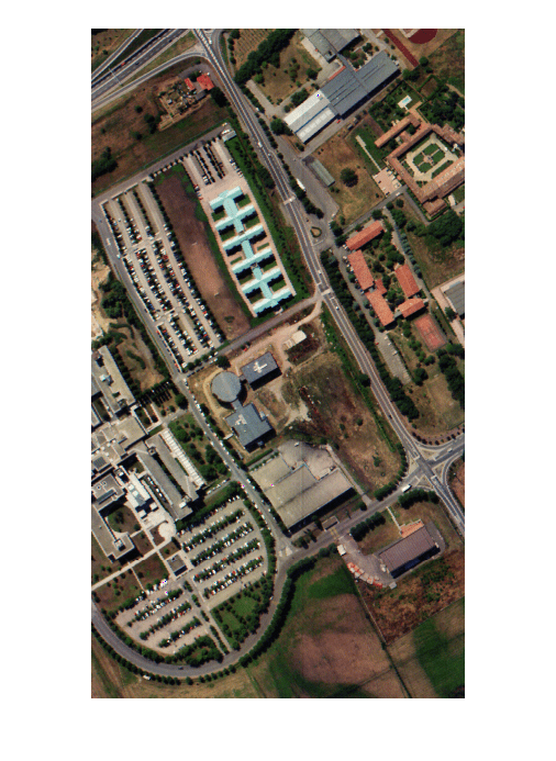

The test data contains the endmember signatures of nine ground truth classes. Each column of sig contain the endmember signature of a ground truth class. Create a table that lists the class name for each endmember and the corresponding column of sig.

num = 1:size(sig,2);
endmemberCol = num2str(num');
classNames = {'Asphalt';'Meadows';'Gravel';'Trees';'Painted metal sheets';'Bare soil';...
              'Bitumen';'Self blocking bricks';'Shadows'};
table(endmemberCol,classNames,'VariableName',{'Column of sig';'Endmember Class Name'})

ans=9×2 table
    Column of sig      Endmember Class Name  
    _____________    ________________________

          1          {'Asphalt'             }
          2          {'Meadows'             }
          3          {'Gravel'              }
          4          {'Trees'               }
          5          {'Painted metal sheets'}
          6          {'Bare soil'           }
          7          {'Bitumen'             }
          8          {'Self blocking bricks'}
          9          {'Shadows'             }

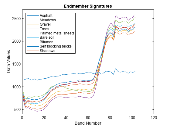
Plot the endmember signatures.

figure
plot(sig)
xlabel('Band Number')
ylabel('Data Values')
ylim([400 2700])
title('Endmember Signatures')
legend(classNames,'Location','NorthWest')

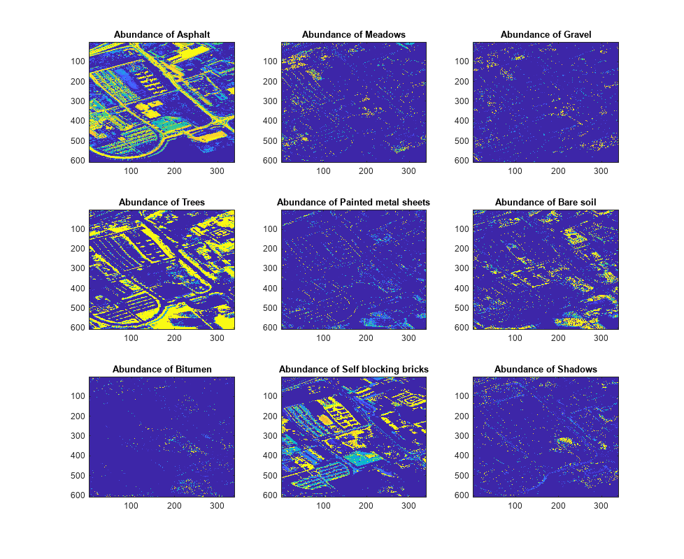
Estimate Abundance Maps

Create abundance maps the endmembers by using the estimateAbundanceLS function and select the method as full constrained least squares (FCLS). The function outputs the abundance maps as a 3-D array with the spatial dimensions as the input data. Each channel is the abundance map of the endmember from the corresponding column of signatures. In this example, the spatial dimension of the input data is 610-by-340 and the number of endmembers is 9. So, the size of the output abundance map is 610-by-340-by-9.

abundanceMap = estimateAbundanceLS(hcube,sig,'Method','fcls');

Display the abundance maps.

fig = figure('Position',[0 0 1100 900]);
n = ceil(sqrt(size(abundanceMap,3)));
for cnt = 1:size(abundanceMap,3)
    subplot(n,n,cnt)
    imagesc(abundanceMap(:,:,cnt))
    title(['Abundance of ' classNames{cnt}])
    hold on
end
hold off

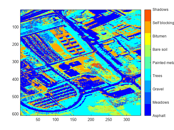
Perform Maximum Abundance Classification

Find the channel number of the largest abundance value for each pixel. The channel number returned for each pixel corresponds to the column in sig that contains the endmember signature associated with the maximum abundance value of that pixel. Display a color coded image of the pixels classified by maximum abundance value.

[~,matchIdx] = max(abundanceMap,[],3);
figure
imagesc(matchIdx)
colormap(jet(numel(classNames)))
colorbar('TickLabels',classNames)

Segment the classified regions and overlay each of them on the RGB image estimated from the hyperspectral data cube.

segmentImg = zeros(size(matchIdx));
overlayImg = zeros(size(abundanceMap,1),size(abundanceMap,2),3,size(abundanceMap,3));
for i = 1:size(abundanceMap,3)
    segmentImg(matchIdx==i) = 1;
    overlayImg(:,:,:,i) = imoverlay(rgbImg,segmentImg);
    segmentImg = zeros(size(matchIdx));
end

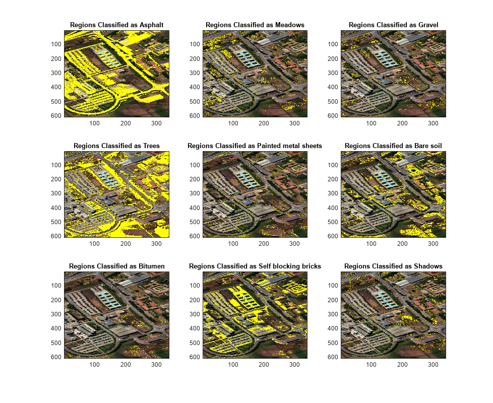
Display the classified and the overlaid hyperspectral image regions along with their class names. From the images, you can see that the asphalt, trees, bare soil, and brick regions have been accurately classified.

figure('Position',[0 0 1100 900]);
n = ceil(sqrt(size(abundanceMap,3)));
for cnt = 1:size(abundanceMap,3)
    subplot(n,n,cnt);
    imagesc(uint8(overlayImg(:,:,:,cnt)));
    title(['Regions Classified as ' classNames{cnt}])
    hold on
end
hold off