imdiffusefilt

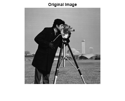
Read an image into the workspace and display it.

I = imread("cameraman.tif");
imshow(I)
title("Original Image")

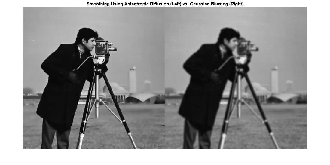
Smooth the image using anisotropic diffusion. For comparison, also smooth the image using Gaussian blurring. Adjust the standard deviation sigma of the Gaussian smoothing kernel so that textured regions, such as the grass, are smoothed a similar amount for both methods.

Idiffusion = imdiffusefilt(I);
sigma = 1.2;
Igaussian = imgaussfilt(I,sigma);

Display the results. Anisotropic diffusion preserves the sharpness of edges better than Gaussian blurring.

montage({Idiffusion,Igaussian})
title("Smoothing Using Anisotropic Diffusion (Left) vs. Gaussian Blurring (Right)")

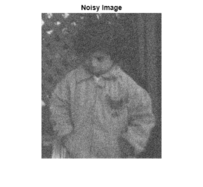
Read a grayscale image, then apply strong Gaussian noise to it. Display the noisy image.

I = imread('pout.tif');
noisyImage = imnoise(I,'gaussian',0,0.005);
imshow(noisyImage)
title('Noisy Image')

Compute the structural similarity index (SSIM) to measure the quality of the noisy image. The closer the SSIM value is to 1, the better the image agrees with the noiseless reference image.

n = ssim(I,noisyImage);
disp(['The SSIM value of the noisy image is ',num2str(n),'.'])

The SSIM value of the noisy image is 0.26556.

Reduce the noise using anisotropic diffusion. First, try the default parameters for the anisotropic diffusion filter, and display the result.

B = imdiffusefilt(noisyImage);
imshow(B)
title('Anisotropic Diffusion with Default Parameters')

nB = ssim(I,B);
disp(['The SSIM value using default anisotropic diffusion is ',num2str(nB),'.'])

The SSIM value using default anisotropic diffusion is 0.65665.

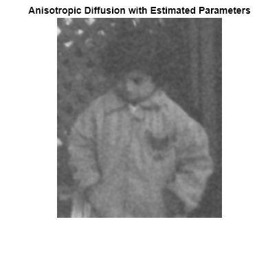
The image is still degraded by noise, so refine the filter. Choose the quadratic conduction method because the image is characterized more by wide homogenous regions than by high-contrast edges. Estimate the optimal gradient threshold and number of iterations by using the imdiffuseest function. Display the resulting image.

[gradThresh,numIter] = imdiffuseest(noisyImage,'ConductionMethod','quadratic');
C = imdiffusefilt(noisyImage,'ConductionMethod','quadratic', ...
    'GradientThreshold',gradThresh,'NumberOfIterations',numIter);
imshow(C)
title('Anisotropic Diffusion with Estimated Parameters')

nC = ssim(I,C);
disp(['The SSIM value using quadratic anisotropic diffusion is ',num2str(nC),'.'])

The SSIM value using quadratic anisotropic diffusion is 0.88135.

Noise is less apparent in the resulting image. The SSIM value, which is closer to 1, confirms that the quality of the image has improved.

Load a noisy 3-D grayscale MRI volume.

load mristack

Perform edge-aware noise reduction on the volume using anisotropic diffusion. To prevent over-smoothing the low-contrast features in the brain, decrease the number of iterations from the default number, 5. The tradeoff is that less noise is removed.

diffusedImage = imdiffusefilt(mristack,'NumberOfIterations',3);

To compare the noisy image and the filtered image in detail, display the tenth slice of both.

imshowpair(mristack(:,:,10),diffusedImage(:,:,10),'montage')
title('Noisy Image (Left) vs. Anisotropic-Diffusion-Filtered Image (Right)')

Calculate the Naturalness Image Quality Evaluator (NIQE) score averaged over all slices in the volume. The NIQE score provides a quantitative measure of image quality that does not require a reference image. Lower NIQE scores reflect better perceptual image quality.

nframes = size(mristack,3);
m = 0;
d = 0;
for i = 1:nframes
    m = m + niqe(mristack(:,:,i));
    d = d + niqe(diffusedImage(:,:,i));
end
mAvg = m/nframes;
dAvg = d/nframes;
disp(['The NIQE score of the noisy volume is ',num2str(mAvg),'.'])

The NIQE score of the noisy volume is 5.7794.

disp(['The NIQE score using anisotropic diffusion is ',num2str(dAvg),'.'])

The NIQE score using anisotropic diffusion is 4.1391.

The NIQE score is consistent with the observation of reduced noise in the filtered image.

References

[1] Perona, P., and J. Malik. "Scale-space and edge detection using anisotropic diffusion." IEEE® Transactions on Pattern Analysis and Machine Intelligence. Vol. 12, No. 7, July 1990, pp. 629–639.
[2] Gerig, G., O. Kubler, R. Kikinis, and F. A. Jolesz. "Nonlinear anisotropic filtering of MRI data." IEEE Transactions on Medical Imaging. Vol. 11, No. 2, June 1992, pp. 221–232.
Extended Capabilities
The imdiffusefilt function fully supports
thread-based environments. For more information, see Run MATLAB Functions in Thread-Based Environment.
Version History
Introduced in R2018aimdiffusefilt now supports thread-based
environments.
See Also
imdiffuseest | imfilter | imgaussfilt | imguidedfilter | locallapfilt | imnlmfilt | specklefilt (Medical Imaging Toolbox)
MATLAB Command
You clicked a link that corresponds to this MATLAB command:
Run the command by entering it in the MATLAB Command Window. Web browsers do not support MATLAB commands.
选择网站
选择网站以获取翻译的可用内容,以及查看当地活动和优惠。根据您的位置,我们建议您选择:。
您也可以从以下列表中选择网站:
如何获得最佳网站性能
选择中国网站(中文或英文)以获得最佳网站性能。其他 MathWorks 国家/地区网站并未针对您所在位置的访问进行优化。
美洲
- América Latina (Español)
- Canada (English)
- United States (English)
欧洲
- Belgium (English)
- Denmark (English)
- Deutschland (Deutsch)
- España (Español)
- Finland (English)
- France (Français)
- Ireland (English)
- Italia (Italiano)
- Luxembourg (English)
- Netherlands (English)
- Norway (English)
- Österreich (Deutsch)
- Portugal (English)
- Sweden (English)
- Switzerland
- United Kingdom (English)